Many types of machine learning problems that can be solved with different algorithms in the Supervised or Unsupervised section. Regression problems are used to create models with Linear Regression, Decision Trees, and other methods that can be used to predict values. We call this a classification problem when we have to group data into predefined groups; logistic Regression and Support Vector Machines are the options. Supervised learning is required for all such models.
Clustering problems can arise when the segmentation of data is required. These can be solved using methods like K-means and DBScan. Methods such as Principal Component Analysis and Factor Analysis can also be used to optimize data. These algorithms are unsupervised.
In both cases, however, we do not consider the time factor when Time Series comes in.
Time series models are used to predict the values over time, i.e., forecasting values.
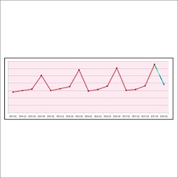
Here are four blogs. The first blog, ‘Introduction to Time Series Data,’ discusses the types of data we encounter when performing time series. It also explores the different characteristics of time series data. The second blog, ‘Averaging Techniques”, focuses on the most basic methods to solve forecasting problems. The third blog, ‘Smoothening and Time Series Decomposition,’ explores medium-level techniques. While the fourth blog, ‘ARIMA family,’ focuses on a collection of more complex methods that are part of the ARIMA family. These can be used to solve forecasting problems.

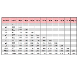
If there is a time factor in the data, a different method must be used to analyze it. There are many data types with a time component, including Panel Data, Cross-Sectional Data, and a mixture of both. This data can consist of four components: Trend, Seasonality, Cyclicity, Irregularity, and Cyclicity. This blog will explain the characteristics of time series data.

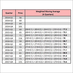
A few methods can be classified as “Level-I” techniques for time series analysis. Many types of averaging models can be used to analyze time series. We will look at three averaging models: Simple Average, Moving average, and Weighted moving average. A simple average uses the mean of an independent variable as the forecasted value. In weighted and moving-weighted average weights are assigned to observations in order to arrive at the forecasts.

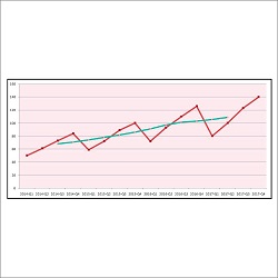
Smoothing Techniques, Time Series Decomposition, and other techniques are classified as “level-II” forecasting methods. Exponential Smoothing Techniques, also known as ETS Model, is a method in which the forecasted value of a time period is a function of both past value and past time period error. The most popular ETS Models include Single Exponential (double and triple exposure), Double Exponential (double and triple exposure), and Triple Exponential (triple). On the other side, Time Series Decomposition uses the components of Time Series Data for forecasting.

A few methods can be classified as “Level-I” techniques for time series analysis. Many types of averaging models can be used to analyze time series. We will look at three averaging models: Simple Average, Moving average, and Weighted moving average. A simple average uses the mean of an independent variable as the forecasted value. In weighted and moving-weighted average weights are assigned to observations in order to arrive at the forecasts.
