There are a variety of new regression techniques that are more suitable than the standard Linear and Logistic Regression. As we have discussed in Linear Regression, we employ an Ordinary Least Square (OLS) method to calculate the unknowable parameters. However, it is an outdated method, and more modern and sophisticated techniques like regularization methods could be employed to construct Linear and Logistic Regression models.
It is crucial to realize at the start that regularization techniques do not help in your ability to learn about these parameters; instead, they aid in the generalization process (i.e., improve the precision that the model can be used when dealing with unknown data) that is done through penalizing complexity (complexity is due to overfitting, where the model is able to remember the patterns of data and then assumes that there are no patterns).
In order to ensure that the model is less susceptible to the inclusion of noise and other particularities in generalization, the regularized regression model can be employed. The main reason for the model to become extremely complicated is due to the model being dependent on too many functions and handling data in extremely large dimensions, and these sophisticated regression models can be employed.
Limitations of OLS
The formula for an easy linear regression model is Y = B0 + B1X1 +E, where B0 stands for the intercept. The independent variable is X1, B1 acts as the covariance, and E represents the term that causes an error. Through this equation, we obtain the Y, which is the predicted value, and by using Y, we are able to know E, which is the value that has to be reduced, i.e., the error in prediction between the measured and predicted value. This error term is crucial since every value that is predicted is not accurate and could be different from what is actually observed, and the term error is used to rectify this gap. This is the place where OLS comes in, as it seeks to minimize the error, which it accomplishes by determining the regression line that minimizes the error (below, we will see at the backend, the software tests different regression lines (Red lines) and then chooses the one that has the lowest sum of the square error (the difference between the predicted value the seen) (Black lines)).
Therefore, OLS, when measured visually, can be defined as the product of distances that exist between every data element and its predicted data point in the direction of the regression line, and it is established in a manner that this OLS is minimal.
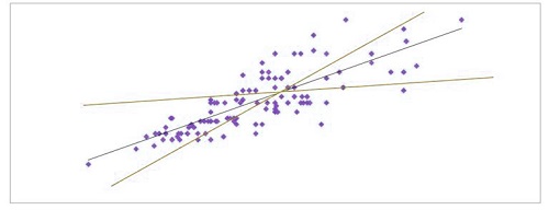
When using OLS, the best line is the one that provides the minimum distance between the actual data points and the predicted points.
We have been using an estimate of the square errors to show the error we have in our “OLS Regression Model’. However, it is crucial to know more about the error. The prediction error is divided into two categories: error due to bias and error due to variance.
To comprehend these sub-components of error, we need to discover the various causes of errors. The root causes of these errors are rooted in the concept of generalization, which is basically a way of generalizing the data we’ve previously observed in a different data set. So when we create models, we do not have two objectives to determine how accurate the model is and how efficient the model is when working when using untested data. These two concepts are fundamentally in opposition to one another. For instance, when we attempt to improve the accuracy of our model, it decreases its generalizing capabilities. Likewise, when we attempt to make the model more generalization friendly, it will lose the accuracy aspect of the model.
For context, suppose we have a database with the Y variable in two categories: poor and rich. We have 100 independent demographic characteristics ranging from their residence location to whether they are wearing spectacles or not. Suppose we could improve the precision of the model. In that case, we can actually make our model remember the patterns that we have in our database and end up storing patterns that, in actual reality, are not useful in determining the financial condition of a person, for instance, whether males sport a mustache or not, or their food preferences, and so on. This creates the problem of overfitting, in which we see excessive patterns and patterns that exist in randomness, possibly due to some kind of noise in the data. Therefore, if we have an extremely high level of complexity, it implies that we have a high variation.
To improve the situation to make the situation better, let’s suppose we use only one feature. This can result in very high bias and extremely low variance. This comes with its own set of issues since, by only having one attribute to apply, we create the assumption that we know everything about the data. If we decide to generalize our data on the base of the region in the country, but this is an extremely large assumption, it could result in a poor precision of our model, leading our model not to be able to fit.
To increase the accuracy of the model To improve the accuracy of our model, we create a more complex model by adding a new feature like their academic credentials. By adding another feature, we can reduce our Bias while increasing the variance; however, if we follow the flow too long and continue to add features, we’ll end up back in the same place we started from, i.e., with a high variance but low bias. It means that a tradeoff exists between the two. We have to determine the “sweet point at which the model isn’t too biased (causing underfitting and causing the model to arrive at an easy solution that is unlikely to be very useful) and also does not have too much variance (causing overfitting in which patterns within the data set are memorized but may not occur and could just be just by chance).
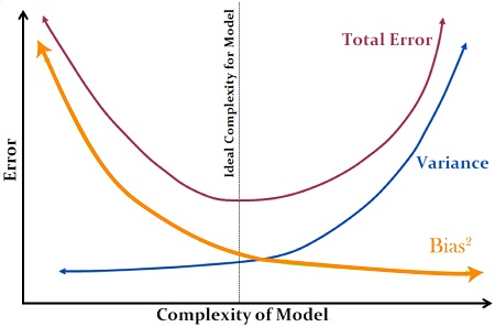
Mathematically, the estimate’s mean square error is the sum of the square of bias plus variance. If we examine the picture above, we can see how, with increased complexity, the bias reduces, and vice versa. The optimal line is between, where the Total Error decreases to the minimum and the growth in bias are the same as the reduction in variance.
The question now is, what is the reason OLS isn’t the best method? According to the Gauss Markov Theorem- ‘among all unbiased estimates, OLS has the smallest variance.’ This implies that OLS estimates have the least mean square error without bias. However, we could have an inaccurate estimate that could be even more lenient in mean square error. For this, we need to make use of shrinkage estimators that analyze the equation for regression to replace the coefficients (Beta-K) with Beta’-K, which results in a lower value than the initial coefficient.
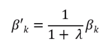
This is the original coefficient multiplied by a term that equals 1 divided by plus lambda. If lambda is zero then we get the initial coefficient, but if the parameter becomes large the output value will get lower, and it can reach the minimum value, which is zero. This will be the estimator of shrinkage, which can provide us with a higher (lower) mean square error. To calculate how much lambda is worth, we apply a formula, and without going into the intricacies of the math that underlie the formula, the way it works is to determine the extent to which a coefficient is greater than its variance, causing it to output (lambda) to be lower. The lambda, therefore, can end the coefficient (making it null) or keep the coefficient but reduce it.
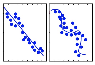
Below, we can see models’ complexity increases when you create the OLS Polynomial Regression Model using 15 features (Right) instead of just one attribute (Left). An increase in the number of features adds complexity to the model. Additionally, it begins to be influenced by less significant features and attempts to account for even smaller variations. Therefore, the significance of coefficients
will also increase due to the increasing model’s complexity.
To manage how complex the model is and counter multicollinearity, we utilize other regression models that can be regularized. In this blog, three kinds of Regularized Regression Methodologies for modeling are discussed: Ridge Regression, Lasso Regression, and Elastic Net Regression.
Ridge Regression
Ridge Regression can be used to construct regularized models where constraints are included in the algorithm to penalize the coefficients that are too big and prevent the models from growing overly complicated and leading to overfitting. In layman’s terms, it is a way of adding an additional penalty to the equation in which w is the vector of coefficients for the model that is the L2 norm, and a is a variable free parameter. The equation is then made to appear to be.
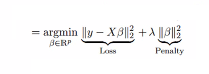
In this case, the first component is the term with the lowest square (loss function), and the second component will be the penalty. When using Ridge Regression, L2 regularization is performed, which adds penalties equal to the size of the coefficients. In Ridge regression, the L2 norm penalty that can be described as ani = 1w2i adds to loss functions, thus penalizing betas. Since the coefficients are squared in the penalty function, the penalty component produces a different result than the L1 norm that we use for Lasso Regression (discussed below). The alpha has a significant part in this as the value of it is determined in accordance with the model you intend to explore. If we decide to take alpha as zero, it will be Ridge, and alpha = 1. It can be described as LASSO, and anything that falls between 0 and 1 is called Elastic Net.

That leaves us with the most important aspect of the equation: to choose what value to assign the parameter that can be tamped Lambda. If we use a small lambda number, the result will be exactly that of the OLS Regression, so there will be no generalization. However, if we choose to use too high of a lambda number it will broaden too much, pulling down the coefficients of many of the features to extreme minimal values (i.e. towards 0). Statistics employ methods like Ridge Trace, which is a diagram that illustrates the coefficients of ridge regression as a function of lambda. We determine the value of lambda that stabilizes the coefficients. Methods like cross-validation and grid searches to identify the optimal lambda to fit our model.
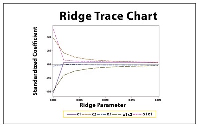
Ridge utilizes L2 regularization, which forces coefficients to be distributed more evenly. It does not cause any coefficient to shrink until it is zero. However, L1 regularization forces the coefficients of the less crucial aspects to zero, leading us to that Lasso Regression.
Note that Ridge Regression can or might not be considered as a Method of Feature Selection method because it reduces the magnitude of coefficients and, unlike Lasso, does not render any variables obsolete that could be described as a legitimate feature Selection method.
Lasso Regression
Lasso is the same as Ridge; however, it performs L1 regularization that introduces an additional cost and = 1|wi| to the loss function, adding penalties equal in absolute values of coefficients, not the coefficients’ square (used for L2); thus causing the weak features to have coefficients of zero. By applying L1 regularization, Lasso makes an automatic feature selection in which the features with zero as their coefficients value are removed. The value of lambda is vital because if its value is too high, it will drop many variables (by creating small coefficients to change to zero), rendering the model too general, which causes the model to be insufficiently fitted.

We can produce a light output using the correct value for lambda, where certain non-essential features are included with zero coefficients. The variables are able to be eliminated, and variables that have coefficients of non-zero can be picked, which will facilitate the model selection.
ElasticNet Regression
Elastic Net is a blended combination of Ridge and Lasso Regression, as it makes use of L1 and L2 regularization. It can be advantageous when many aspects are linked to one another.

In the above equation that both L1 as well as L2 (||.||1 and ||.||2) are used to regulate the model.
Therefore, these regularized regression models can be used to determine the right relationship between dependent and independent variables by regularizing the independent variable’s coefficient. They aid in reducing the danger of multicollinearity. Regularization of certain regression models can be problematic if the features of the independent variables are not linearly linked to the dependent variables. To address this issue, it is possible to transform the features to ensure that linear models like Ridge and Lasso are still applicable, for example, applying polynomial basis functions to linear regression. The transforms allow a linear regression model to discover the polynomial or non-linear relationships within the data.
