One-way ANOVA is used to examine the mean of groupings of the independent variable to determine whether the groups are distinct from each other or not. It is crucial to remember that an independent T-Test can also be utilized when the variable is independent and is only two degrees (groups). The only difference between T-Test and One-Way ANOVA is that the T-Test produces the T value, whereas ANOVA will yield an F Ratio that is nothing more than the T value multiplied by the square; however, the results will be the same. The T-Test is not utilized if the levels of the independent variable are greater than two. In the case of an independent variable that has three levels, namely X, Y, and Z Then, we need to test three times to compare X to Y, Y with Z, and Z with X, and every time we test, i.e., the more times, it takes to run the test and the more likely it is that we will make an error of the type I increase.
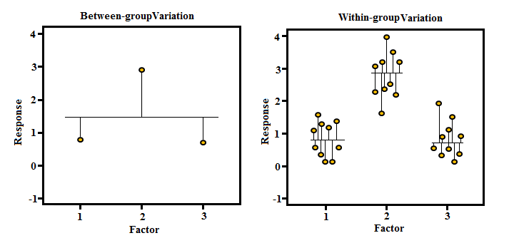
In relation to the One-way Analyse of Variance, one of its purposes is to check whether the means of groups are equivalent. To do this, we calculate an F ratio, in which you divide by the variability of an independent variable in two parts Variation between the means of each sample and variations within the samples, i.e. the variance that results from differences between groups and variance attributable to within-group variations within the group. In One-Way ANOVA, the F-statistic is represented by the following ratio:
F = variance between sample means ÷ variation within the samples.
Introduction to F Ratio
Prior to getting specific about how we determine how we calculate the F Ratio, it is important to be aware of the reason we divide the difference between the groups and also the variation between the groups. To grasp this, let’s look at an illustration.
Imagine that you’re the clothing shop owner and decide to launch the Diwali promotion where you randomly select 1000 from your clients and then categorize them into three categories. The first group will comprise customers who have spent, on average, Rs.10,000 at your store; you will receive a gift card of 1,000 rupees. Similar to Group II and III, those who have spent Rs. 5,000 and Rs. 1,000 at your store. You will receive a gift card amounting to Rs. 500 and Rs. 100, respectively. Before deciding on the offer, you need to ensure that the groups have a purpose and, therefore, determine whether these groups are (statistically) distinct from one another when you look at the first group and find that customers from the first group are required to spend a specific amount of money like this:
20000, 6000, 12000, 4000, 8000 etc . If we look closely, the average would be just 10,000 (20000 + 6000 + 12000 + 4000 + 8000 / 5 = 10000). However, the values vary greatly, so the groups aren’t meaningful; however, if the sample contained numbers such as 10000, 9000, 13000, 10000, and 8000, this group could have been made to make more sense because the variation within the group would have been lower. For this Group I is to remain different from Group II, the variation between the two groups must be substantial. Therefore, to say that the distinction between two groups has significance, it is necessary to have a significant variance between the groups has to be small; however, the variance between groups must be large, and this is the formula for the F-statistic utilized to calculate the One-way Analysis of Variance that is the ratio of the variance between the means of each sample and the variation in the sampling.
Calculation-
The formula used to determine the F ratio in statistical terms is F ratio in terms of statistics is

This is basically:

In this case, the Numerator can be described as that of the Mean Square between the group (what we’ve been calling finding the variations between the different groups), and the denominator is what we call the Mean Square Error, also known as the Mean Square Error within groups (what we’ve been referring to as the finding of the variance between different groups). ANOVA examines whether the amount of variance (variance) discovered between groups is small or large when compared with the average amount of variance (variance) observed between the groups. The method used to calculate the F Ratio is comprised of:
Step 1: Identifying the average of the variation within each of our samples (levels)(MSb) – the Mean Square Between (MSb)
Step 2: Finding the average variance within the samples (levels) – Mean Square Error Within (MSwithin) is also known by the name of Mean Square Error (MSe).
Step 3: Once MSb along with MSe are determined, you can divide them to calculate the F value.

The variance between the groups v/s Variance within the groups
Formulating MSb (Mean Square between) (Numerator of F Ratio)
Contrary to the numerator for T value that simply determines the difference between two means, ANOVA requires finding the mean difference since there could exist more than two different groups (levels) in an independent variable. Therefore, finding the average difference between the sample’s mean is necessary.
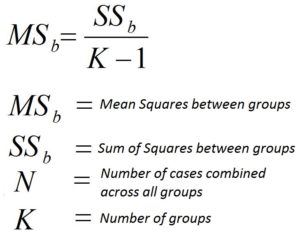
The formula to calculate MSb is the following formula: MSb will be SSb divided by the degree of freedom SSb.

Finding the Numerator of MSb (SSb)
Here, SSb represents the total squares between the two groups, which can be calculated using
Step 1: subtract the Grand Mean (Mean of an independent variable) from the group’s mean.
Step 2: Square these deviation scores
Step 3: Multiply each squared deviation by the number of cases within each group.
Step 4: Add the squared deviations of each group.
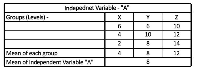
Example: An independent variable named A with levels (groups) X, Y, and Z

Step 1: Determine the average of A and the mean of the groups X, Y, and X.
Step 2: Subtract the group’s mean with the grand mean and then square it.
Step 3: Perform the steps above for each situation within the group.
Step 4: Add up all values
e.g.- (4-8)2 + (4-8)2 + (4-8)2 + (8-8)2 + (8-8)2 + (8-8)2 + (12-8)2 + (12-8)2 + (12-8)2 = 96.
Here, our SSb appears to be 96.
Finding the MSb denominator (degrees of freedom SSb)
To determine how many degrees of freedom are available to calculate the degrees of freedom for SSb, We subtract the total number of levels (groups) within each independent variable by 1 (K-1 with K being the number of levels that are in the independent variable).
We now have the numerator as well as the denominator of MSb We simply have to divide the SSb by the degree of freedom i.e.
96 / (3-1) = 48
This is why we have MSb as 48.
It is important to remember that MSb is the measure of the variation between groups. As per the case (Diwali provide an example), we would like that the variance be large, suggesting that Group I, II, and III differ from one another and, for this group, means shouldn’t be placed close to the mean of the entire group as if they were, it means they have a small variance. However, if the group’s means are distributed away from the means (mean of an independent variable), the variance between groups is greater.
Calculate Mean Square Error Within (MSe or MSwithin) (Denominator of F Ratio)
We can determine how much the meanings of the group differ from the independent variable mean; however, as we have seen in one of these examples, the different levels or groups will have less variation for us to continue with the Diwali offer. To do this, we have to figure out how far every observation is from all observations’ averages. In contrast to the differences between the numerator of the t value and f value, the denominator of the faction in the T-Test as well as the denominator for the value of F (which corresponds to the means square error within) is nearly identical to that in T-Test. The denominator represents the standard error in the difference between the two sample means, and the MSe (denominator of the F value) is the square of average errors in each group (i.e., the variation in average between the two groups).

Finding the Numerator of MSe (SSe)
Here, SSe is the total of square error within the groups, which can be calculated using
Step 1: Subtract the mean of the group by each score
Step 2: Square the value above-calculated
Step 3: Add all such values
Step 4: Repeat this for all groups and add them to arrive at a final number.
Example: have an independent variable A that has levels (groups) Z, X, and Z.

Step 1: Determine the average for variable A as well as the mean of the groups Z, X, and X.
Step 2: Subtract the amount of a group from the mean of the group and divide it by.
Step 3: Repeat the same step for every situation within the group.
Step 4: Add up all values
e.g.- (6-4)2 + (4-4)2 + (2-4)2 + (6-8)2 + (10-8)2 + (8-8)2 + (10-12)2 + (12-12)2 + (14-12)2 = 24
Finding the common denominator between MSe (degrees in freedom of the SSe)
Degrees of Freedom for SSe can be calculated by using the number of cases within each group and subtracting 1 out of each group. Or, in other words, it’s N-K. The number N represents the total number of cases across all groups, and K is the overall number for all the groups. (Notice that this formula is nearly similar to the formula for degrees of freedom utilized for the T-Test for independent samples).
We now have the numerator and denominator of MSe We just divide SSb by its degree of freedom i.e.
24 / (9-3) = 4
SSb v/s SSe
* SSe subtracts the mean group from the individual score for each group. SSb subtracts the grand means (independent variables mean ) from each groups’ mean.
* SSb divides every squared deviation by the number of cases within each group and provides us with an approximate variance between the group’s mean and the mean grand for every instance in each group. SSe subtracts the Group Mean by the score of each individual is squared and then adds them up after doing this for all groups.
Degrees of Freedom SSb vs. Degrees of freedom of SSe
K refers to the total number of groups. N is the total number of samples of the independent variable.
In order to convert SSb to MSe, it is necessary for the SSb to be divided by its degrees of freedom, which in this case is K-1 (df=K-1). In contrast, when we want to convert SSe to MSe, then we must divide SSe in accordance with the degrees of freedom (which is the number of samples for each group with each one of them subtracted by one) and, after doing this across all groupings, we need to add them all up ((n1-1) + (n2-1) + (n3-1 )…) or we can subtract the total numbers of the groups using the total number of samples (N-K)
SSb + SSe = Sum of Squares Total (SSt)
If we combine SSb and SSe and SSe, we will arrive at the total sum of squares (SSt), the total variance across the whole data set. To comprehend this, we can look at another illustration.
Example: Create an independent variable named A with levels (groups) such as X, Y, and Z.

Step 1: Determine the mean of A and the mean of the three groups, X, Y, and Z.
Step 2: Subtract the values of each group by your grand mean (mean of an independent variable).
Step 3: Round the result of the previous step (to get rid of all negatives).
Step 4: Repeat the same step for every situation within the group.
Step 5: Combine all values
e.g.- (6-8)2 + (4-8)2 + (2-8)2 + (6-8)2 + (10-8)2 + (8-8)2 + (10-8)2 + (12-8)2 + (14-8)2 = 120.
It is interesting to note that The SSb and SSe that were generated with this dataset was 24 and 96, respectively, and when you add them up, the result is expected to be 120, which is the number we use for our SSt.
Calculating F Ratio

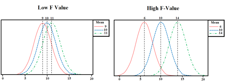
High v/s Low F-value
This F-statistic represents what is known as the percentage of the variance between the Means of the Samples and Variation Within the Samples. Their values are anticipated to be approximately similar in the absence of an assumption of the null hypothesis (i.e., that the two groups are identical and share the same mean), creating an F-statistic, which is close to 1. F Raito is very useful since it encompasses both variations discussed in the preceding sections. If F values are large, the variance of groups is significant compared to the within-group variability. In contrast, If you find that the F value is very small, i.e., close to 1, it implies that the variance between the groups is minimal as well as within the same group, it is high. If we want to disprove the null hypothesis that the mean of the groups are the same, we require a high F-value. (Unlike that of the value P, where when you find that the value of P is large in comparison to our significance level that is usually set at 0.05 or less, then this means that the Null Hypothesis can be accepted). In the previous example, the F Ratio works to 12. (MSb/ MSe = 48/4)
However, the issue is what the maximum F-value must be to eliminate the null hypothesis. This we have been discussed in the following section.
Using F Statistic for Hypothesis Testing
Suppose you consider that the Null Hypothesis proves true. In that case, i.e., the mean of the two groups is equal; if the Null Hypothesis is true, the F stat (which refers to the ratio between the variance within the group and in the particular group) results in an F-Distribution.

To determine how statistically significant the difference in the mean of the group is, we need to determine the F value on the F Distribution to see if our conclusion is within the critical area within the F Distribution. The higher the F value, the stronger evidence we have to support that Null Hypothesis. The next step is to calculate the likelihood of having an F value just by chance. To calculate the probability of placing our F value onto the F Distribution (when the Null Hypothesis is true, the F statistic has an F Distribution), and this F distribution is determined by the degree of freedom we have in the numerator and factor of the denominator for the F Ratio. Then, when we graph your F-statistic, we will find the likelihood of having an F value is based on chance, i.e., having an F value or an amount that is higher than this is the area of the curve (i.e., an area right to what we have calculated as our F). Area under the curve (AUC) is the probability of getting our F number or something else in the right-hand tail. The F table determines the area to the right of our F value. It is important to think about the degree of freedom we had in the numerator as well as the denominator. Then, we can look at through the different p values available to us. We then determine the area to the right side of the curve with various levels of significance (α).
The tables might not give a precise solution, but statistical software can be used to determine the exact p-value. If the p-value is more than our significance level, we will accept the Null, but if the p-value is less than the considered significance level, we reject our Null Hypothesis and can say the F-value is sufficient to reject this Null Hypothesis.
Assumptions for One Way ANOVA
* We presume that this population is evenly dispersed (normally distributed) and the samples are independent.
It is important to remember that the size of the sample and the variation for each group is about the same.
Effect Size
It is important to remember that a point about the statistical significance that was mentioned previously and that having a high statistical significance does not automatically suggest that the result is actually significant. If your sample is extremely vast, even a tiny difference could be determined using the test to be statistically significant. However, in the real world may not be considered a significant alteration. It is therefore important to keep the practical aspects in your mind.
Poc Host Test
One problem of One way ANOVA is that it does not identify the groups that are different in significant ways and which don’t. To test this, the Poc Host test can be performed. There are many types of Poc Host Tests, such as the following:
- Tukey’s HSD Test (HSD: Honestly Significantly Different)
- Duncan’s latest multiple range test (MRT)
- Dunn’s Multiple Comparison Test
- Holm-Bonferroni Procedure
- Bonferroni Procedure
- Rodger’s Method
- Scheffe’s Method
Certain tests are more cautious than others, i.e., making it difficult to form statistically significant groups, but they all adhere to the same basic principles. Each group’s mean is evaluated against each other to determine if they’re distinct from each other.
Priori Contrasts
Priori Contrasts can be used to find the specific groups or groupings that differ from one other in their mean values of the dependent variable. One example could be an independent variable with four groups, namely A, B, X, and Y. They need to know whether A and B differ statistically from X or Y. Priori Contrasts can utilize these variables.
One-way ANOVA aids in comparing the different categories of an individual variable. There are times when there are multiple independent variables, and that brings us to the next topic, Factorial ANOVA.
