Measurements of Shape as a descriptive statistic can help us to determine how numbers of data points in a data set are distributed. It helps us to find the patterns that might be hidden and are easily discernible once the data is displayed on graphs. In this blog, the data, as well as the different shapes that can be found in it, are examined. It is crucial to remember that only specific kinds of data can be explained as the shape of quantitative data, which follows an orderly pattern and has some type of weight. In contrast, qualitative data can’t be used since their values do not have any weight to which they can be attributed.
The form of data can be understood by looking at the distribution of data elements across the space. The distribution can be classified as Symmetrical distribution (e.g., Normal Distribution) and Asymmetrical Distribution (Skewed Distribution). This blog entry explains all of these distributions will be discussed.
Symmetric Distribution
A Distribution could be described as Symmetrical if both parts of it are a mirror image of each other If you can separate it from its mean, the information you see on the left of the distribution is what you will see on the opposite side.
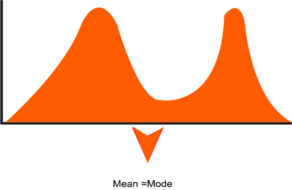
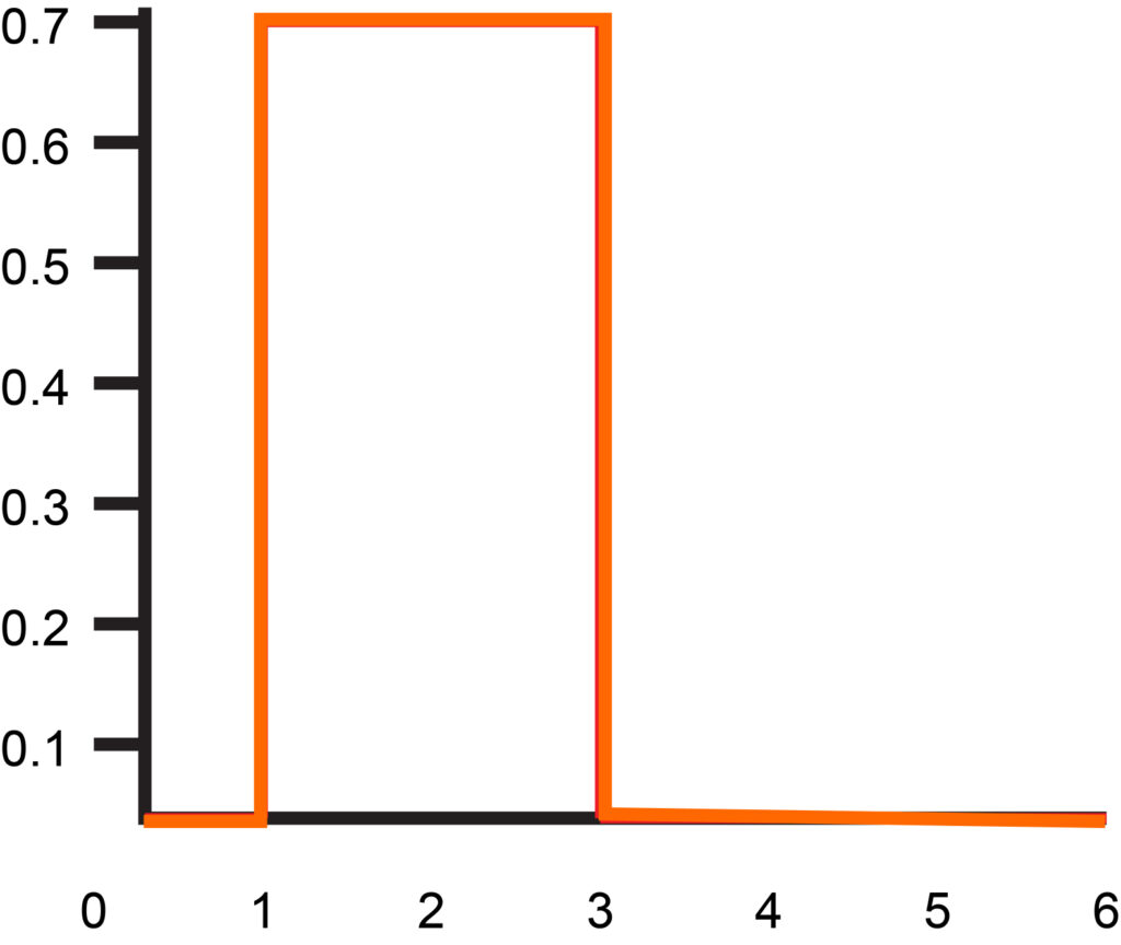
The most common examples of Symmetric distributions are Rectangular distribution, U-shaped distribution, Normal Distribution, Rectangular Distribution, etc.
U-shaped distribution
Rectangular Distribution
The majority of Symmetric distributions have a unimodal structure, i.e., they have a single peak; however, the other kind is multi-modal or bimodal, which has several peaks within the distribution, which means that there is more than one mode within the data set, however, the median and the mean are identical in these kinds of distributions. In the blog article discussed here, there is only one type of Symmetric Distribution addressed: the Normal distribution.
Normal Distribution
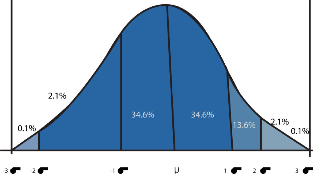
The Normal Distribution is one of the Symmetric Distributions in which the median, the mean, and mode are in line with the other. The most important characteristics to determine a normal distribution or aspects that make a particular normal distribution are as follows:
It is symmetrical; as described in the previous paragraph, the distribution mirror’s left and right sides are split by the middle in which the mean, median, and Mode meet.
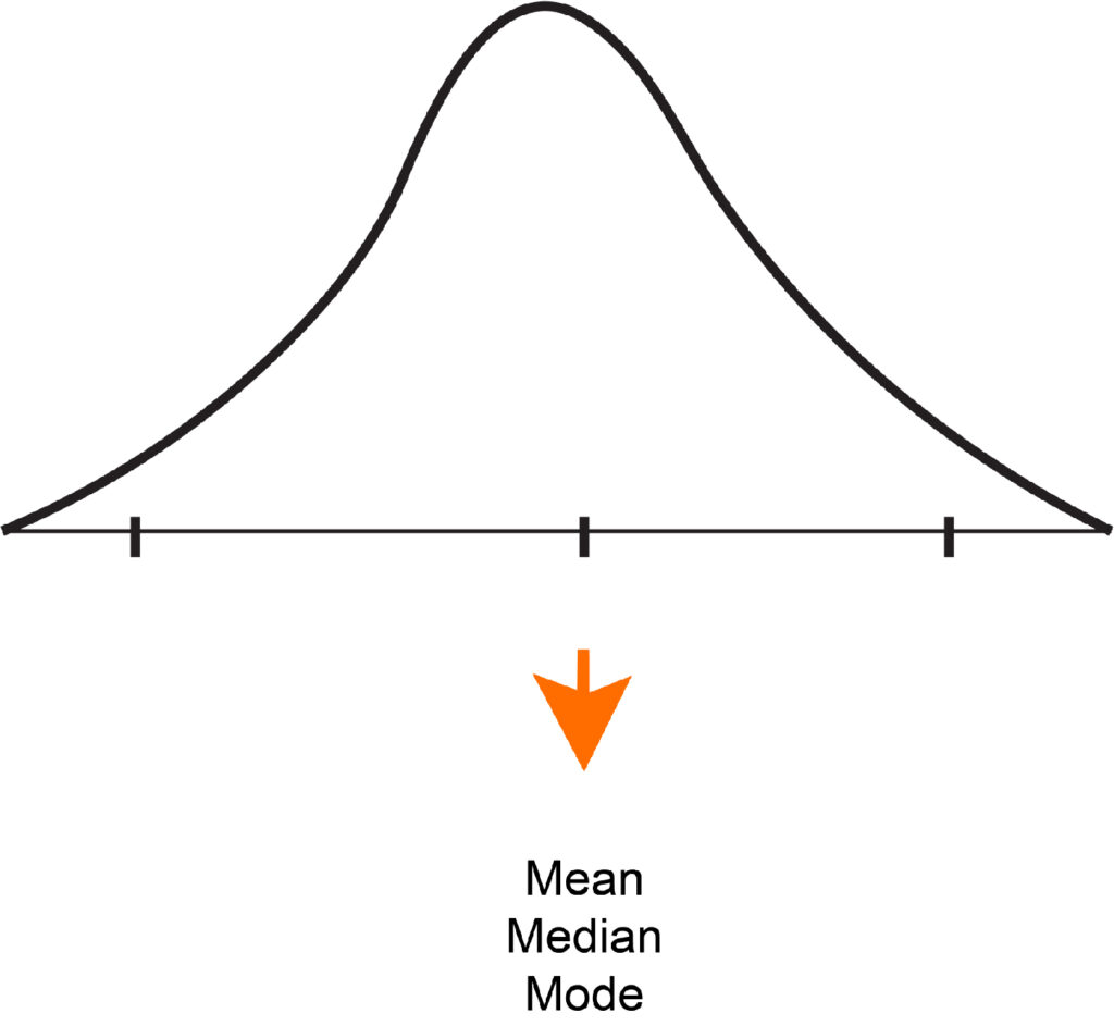
Secondly, The Mean, Median, and Mode coincide in the middle when data is plotted onto a graph. Furthermore, since this distribution is the highest near the center, it exhibits an angular curve if a graph is made. This type of distribution has a unimodal distribution, i.e., the only value repeated for the longest time.
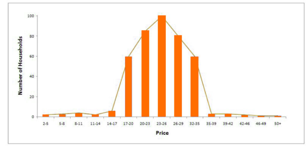
Then, Its tails (upper and the lower) do not meet the bottom (x-axis), thus making it asymptotically distributed (Asymptotic Distribution).
Each of these three aspects that make up the normal distribution is crucial in the field of statistics since they enable us to calculate probabilities. They also play an important role when it comes to Inferential Statistics. If all three characteristics are considered, it is possible to conclude that most of the data lie at the center, and the values become extreme and uncommon when we get away from the center on one or both sides. This leads to an Empirical Rule, or the Three Sigma Rule, that allows us to state that when the data is typically distributed that 68% of values are within a Standard Deviation (the data above and below a standard deviation are the same because it is not symmetrical) 95 percent at 2 and 99.7 percent with 3. Standard Deviations.
Asymmetric Distribution
If the sample data collected is deliberately biased and includes data points with specific characteristics, this can cause the distribution to be Asymmetrical. In Asymmetric Distribution in which the two sides don’t reflect one another.
Skewed Distribution
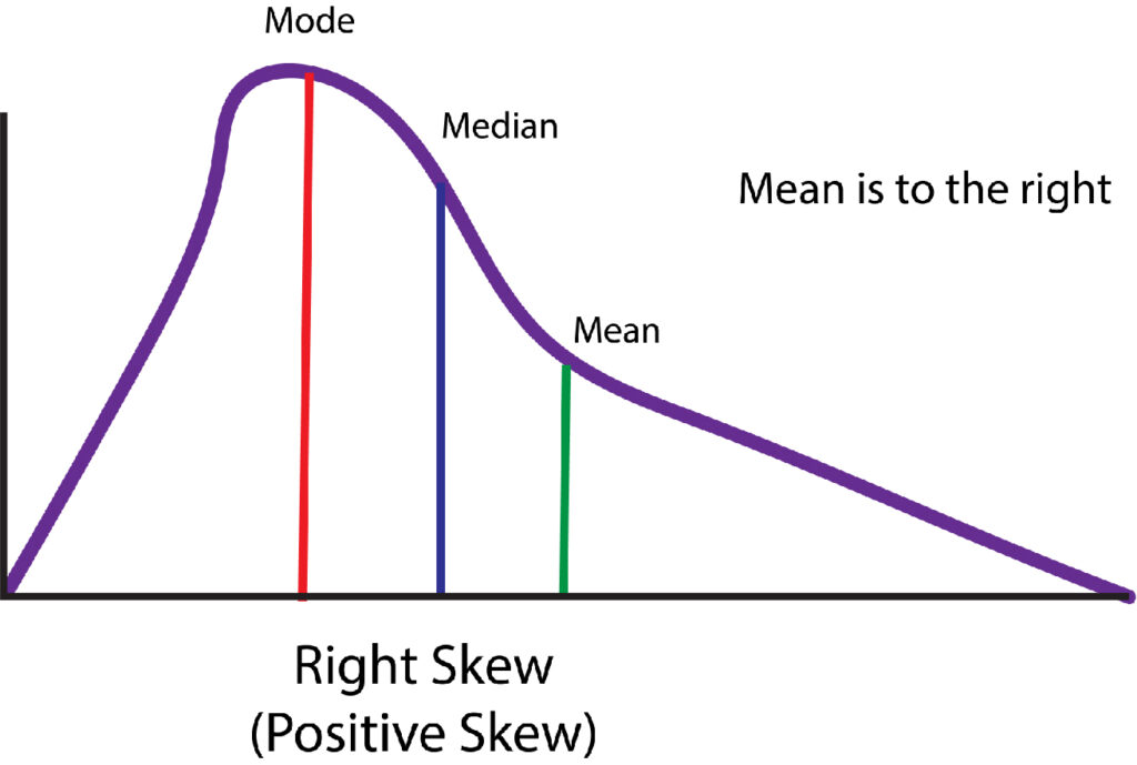
Skew is one of the characteristics commonly used to define what happens to values. When it comes to Asymmetric distributions, the distribution could be skewed either positively or negatively. This occurs when the more common values are crowded between the low and high ends of the x-axis. This is among the most commonly used designs when a distribution is divergent from the normative distribution. In this case, the median, mean, and mode don’t coincide. The easiest method to determine whether the distribution is skewed or not is to make a histogram, then observe the form of the distribution. If it’s skewed, it is either Positively Skewed or negatively skewed.
Positively Skewed Distribution
A distribution is considered to be positively skewed when the median of the spread is greater than the median, and the majority of the scores fall in the lower part of the distribution, while a few scores are on the higher part of the distribution. Any probability based on such an analysis is likely to underestimate the number of scores on the lower end of the skewed one while overestimating the scores on the higher part of the distribution. If we plot the distribution in a histogram, it is evident that the left side will be larger than that on the left one, with the mean located on the right side and the media on the left. This is the reason why Negative Skewed distribution is also known as Right Skewed Distribution. This means that the distribution is positive in the event that its mean value is higher over the median (making the mean to be in the middle of the median). There are a few scores at the lower end of the spectrum, creating an elongated tail on the top that is the highest distribution point.
Negatively Skewed Distribution
A distribution is negatively skewed where the average of the distribution is greater than the mean, and the majority of the scores are at the upper end of the distribution. In contrast, a few scores are located in the lower part. Any probability based on an underlying distribution may underestimate the number of scores on the lower end of the distributed skewed one and underestimate the number of scores on the upper end. If we plot this on a histogram, the left-hand right side will be larger than that on the right one, with the mean to the left side and median on the right. This is why positive Skewed distribution is referred to as the Left Skewed Distribution. This means that the distribution is negative Skewed in the event that the mean is lower than the median (making the mean to the left of the median) and a small number of are at the upper end of the spectrum, making an elongated tail on the lower side of the spectrum.
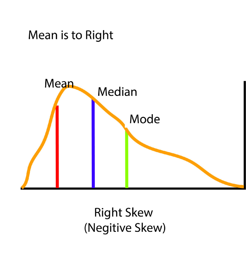
The most common examples of skewed distributions could consist of a test that is a surprise in maths, which, if found to be extremely difficult and causes many students not to score well, and when the scores of the students were plotted on a graph, then the form of the distribution will show an asymmetrical distribution. However, it is the case that the test is found to be extremely simple, and all the students achieve extremely high scores; the distribution will be a Left-Skewed Distribution.

Other Shapes of Distribution
In addition to other than Normal and Skewed distributions, different forms of distribution were briefly discussed in the following paragraphs.
Kurtosis
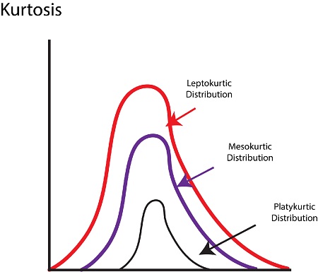
Similar to skewness, Kurtosis is a term used to describe the shape. It defines the form spread in terms of flatness or height. There are several kinds that are affected by Kurtosis: Leptokurtic, Platykurtic, and Mesokurtic.
Leptokurtic
If you have a significant positive over exceed of kurtosis, then the form that the distribution takes is referred to as Leptokurtic. To comprehend this by its shape, it has larger tails. Compared with normal distributions, it has an identical peak (to be exact, this distribution has a greater peak than the one normally found in a bell-shaped distribution and is significantly more so compared to the Platykurtic distribution). Values that are clustered around the center (mean ).
Example: If you’re asked to collect a sample of data to discover the median price of the automobile owned by people throughout Delhi, and you choose to only go to higher-middle-class areas, the distribution of a sample is Leptokurtic.
Platykurtic
Suppose the result is a negative surplus of kurtosis. The shape that the distribution takes is known as Platykurtic.
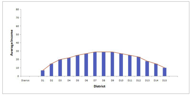
These data elements are dispersed along the X-axis, resulting in shorter tails contrasted with a normal distribution. It has very few values that cluster around the center (mean). This type of distribution has no central tendencies.
Example: You are requested to visit fifteen localities or districts of your city to gather a sample in order to determine the median earnings of your state. You decide to visit each district and calculate the median income for each district by randomly picking 40 people and then calculating the annual earnings of each. However, when the data was displayed on a histogram, the distribution appeared to be Platykurtic as all of the districts you selected to visit were areas housing government households in areas where residents’ incomes were in the middle-income range, with each having the same median income. This caused the distribution to be less rounded than normal.
Mesokurtic
This is the time when you have a normal distribution. The parts of the tail are neither too thin nor too thick, scoring is equally split, and scores are not concentrated around the central point nor too dispersed.
Bi-Modal and Multi-modal Distributions
A normal distribution typically contains one point. It is possible to have a distribution with more than one mode, and in these scenarios, it could become Bimodal (if it has two peaks) as well as Multimodal (if it has more than two peaks). The peaks can indicate different groups that could be present in the data. It could mean it is sinusoidal (a shape with waves).

The shape of the distribution plays an important part because it is the form of the distribution which allows concluding the population from the data samples. Knowing the form of the distribution is essential to understand how inferential statistics operate. The blog in this post explains we will discuss what a normal distribution is and what other designs a data may adopt other than the famous bell-shaped curve, were explored. After you’ve mastered this article, you’re prepared to go on to Inferential Statistics.
