A Measure of variability shows the spread of scores, i.e., it aids us in identifying the variance, the degree of similarity or variation each data point is within an individual or a group.
Before we can understand the various Measures of Variability, it’s important to comprehend the necessity for Measure of Variability if we have a Measure of Central Tendency to explain and summarize our data into one value. As we said earlier, the measurements of Central Tendency can suffer from outliers and the nature of the distribution and thus cannot give a true and impartial view of the data. Additionally, they fail to help us comprehend how dispersed or scattered our data may be and how far they are from the ‘Centre.’
Example
To better understand this, we will look at one example.
If there are two buses within the area you live in, Bus-A and Bus-B, you could choose to travel to your school. It is expected to get to your school at 8:15 and has a limit of 5-10 minutes for being late. Both buses are accessible to you around the same time. However, the issue is which one you should choose to take to get to your school at the right time. In the hypothetical scenario, we have historical records of both buses for the last 10 days, and we can see that both have the same average time of arriving at the school at 8:15.
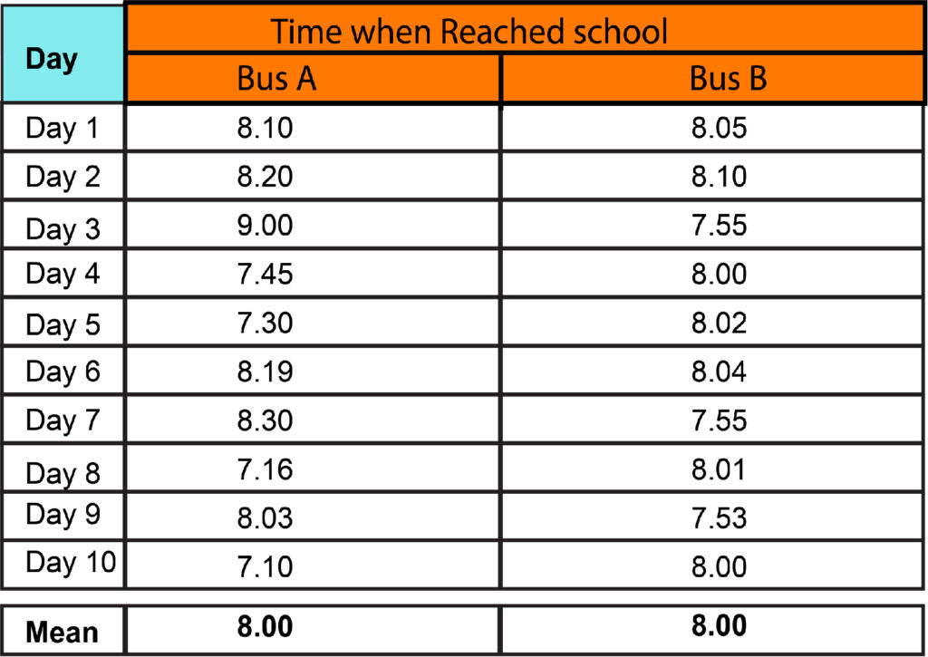
But, if we analyze it, we will see that Bus A is much more unpredictable than Bus B. “Data points” for Bus-A have a greater “Spread Out” than Bus B. This makes Bus B more trustworthy in terms of statistics. The Measure of Central Tendency, be it at Mean Mode, Median, or Mean, does not provide this crucial information. This is the reason the measures from Central Tendency help us.
There are three primary indicators of variability (Dispersion). The three main measures of Variability (Dispersion) are Variance, Range, and Standard Deviation. However, Standard Deviation is the one that is the most frequently used.
Range
The range is the gap between the biggest and the smallest values of our distribution or data.
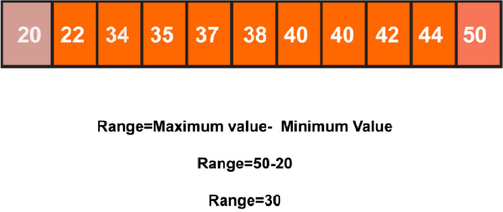
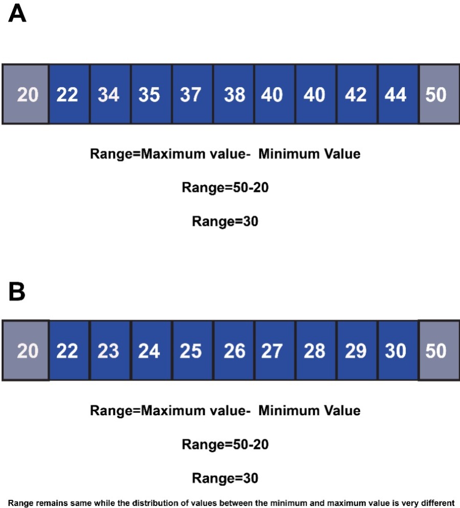
The issue with using ranges is that it is very misleading since it doesn’t clarify the differences between the maximum and minimum values.
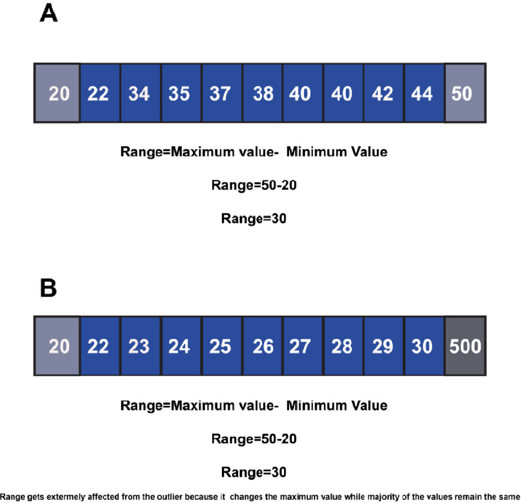
Additionally, Range is highly vulnerable to outliers because they can change the range’s minimum or maximum value.
Quartiles
Quartiles, Quintiles, Deciles, etc., could also be used to determine the extent of the variation of scores in an array of data.
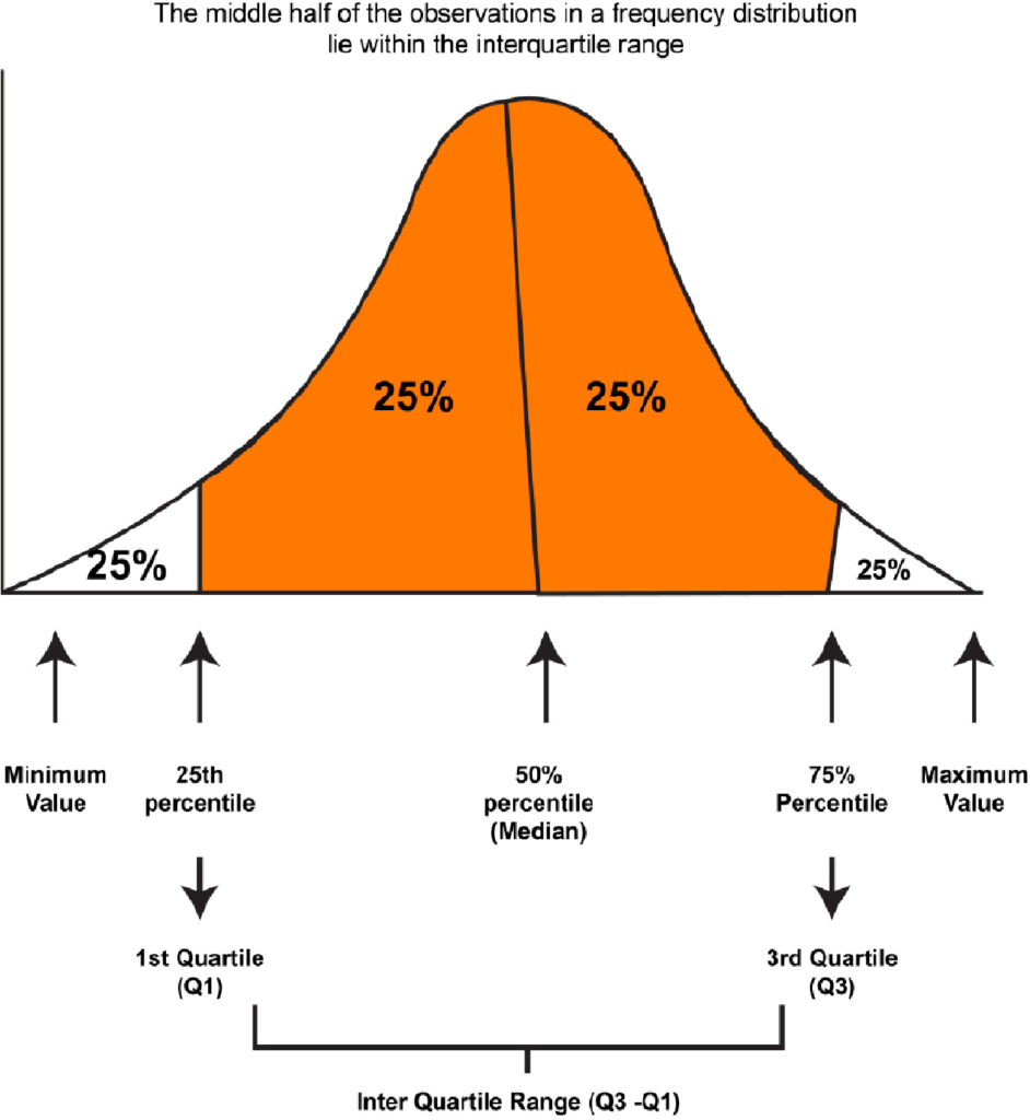
Quartiles break down a data set into four equal parts. They are used to describe the values of the points between the quarters. Quartile 1: The lower Quartile (Q1) Q1 is the area that lies between the bottom 25 percent of values and the most valuable 75. It’s also known as”the 25th percentile. The second Q2 (Q2) represents the midpoint of the data. It’s also known as the 50th percentile, also known as the median. The upper quarter (Q3) refers to the interval between the lowest 75% of values and the top 25 percent of values. It’s also known as the 75% mark.
The Interquartile Range is the difference between the value, which is the 75th percentage (3rd Quartile), and the one considered to be the 25th percentage (1st Quartile), unlike the Range, which is simply what is different between the highest and smallest value. Suppose the values of the distribution are ordered from smallest to biggest and then divided into four equally sized groups. In that case, the Interquartile Range will be the value in the middle of the two Quartiles that describe the middle 50 percent of the values in the distribution. One advantage that Interquartile Range has over Range is that it isn’t affected by outliers, whereas the Range is affected by outliers.
It is absolute that the sum of any deviation must be zero.
For instance, if there is a set of data that has 4 values, namely 45, 64, 68, 51, with a mean of 57, and we attempt to determine the deviation of each of these values from the average by subtracting each value from that of the average (45-57=-12, 53-57=7; 68-57=11; 51-57=-6) and attempt to summarize everything by adding up the results, the result is an unimportant zero (-12 plus 7+11 + 6). Thus, the total of these “deviations” is zero, i.e., the average deviation from the mean will always be 0. This is because the means is simply an equation for the middle point of the spectrum. Naturally, some scores will be higher and below that mean, resulting in negative and positive deviations. When we add all these variances and subtract the negative value, it cancels out the positive ones, leaving us with a zero. In the absence of an average of zero, we employ a different method to solve this issue. We can utilize the Mean Absolute Error (MAD), the most frequently used Variance, which produces Standard Deviation to avoid getting an 0 in the sum as our numerator. Attempt to divide the total of our deviation by the denominator, that is, the number of values within the actual distribution.
Mean Absolute Deviation (MAD)
To address the issue mentioned above, we calculate the Mean Absolute Deviation, i.e., the distance that is the average of the mean. We calculate the mean Absolute Deviation by subtracting every observation by adding the mean of the distances (ignoring the significations since the Mean Absolute Deviation has been calculated taking only absolute values, so the result can always be positive) and then dividing it by the total number of observations.
In our instance, in our case, the MAD (Mean Absolute Deviation) is 9 (13+7+11+7=36 36/4 = 9). Mean Absolute Deviation can be beneficial because it is simple to comprehend and calculate; it provides the average deviations located in our distribution; however, it is susceptible to being subject to extreme values that can alter the mean dependent on it. Additionally, it violates the principle of algebra by not recognizing the + and – signs in calculating the deviations.
Variance
The variance not found in Range or Interquartile Range determines the data distribution within the mean. It shows how much each value in a given data is similar to the median of its distribution. Variance is the average of the distance squared to the mean. It is a different measure of the score, i.e., the middle for the distribution. This also counters the problem previously mentioned, in which the deviation of the mean from the mean always equals 0. To combat this issue, we calculate the squares of deviation from the mean to ensure that the final result isn’t 0. For instance, the variance of the above data set is 71.
The formula for Variance is

where,
S = to sum
X is a score based on the distribution
M = the number of people mean
N is the number of cases within the population
x is the sample mean
N = the number of cases within the sample
Standard Deviation
Although it is a useful statistic, it is usually used as a part of formulating other statistics and generally is not utilized as a standalone stat. Variance is used as a method in the calculation of standard deviation. We use the square root of the variance principally because the numbers have units, and taking squares of those units could yield a different result. For example, if our unit of measurement for our values is in meters, and we attempt to determine the variance of this distribution, then it will result in square meters. Suppose we take an average of square roots for the variances so that negative values don’t overpower each other. In that case, it’s recommended to normalize these values with the square roots of variance. This gives us Standard Deviation by simply taking the square root of the variance. Standard Deviation is commonly used to establish how much variation from the average is considered acceptable within the context of a particular distribution. Additionally, in certain circumstances where two datasets have similar means but differ in standard deviations, it is possible to claim that the one with the highest standard deviation is more “unreliable in comparison to the one with a lower Standard Deviation (as in the example above of two school buses). ).
For instance, our Variance for the above data set would be 8.4.
The formula for Standard Deviation is

where,
S = to sum
X is a score based on the distribution
M = the populace mean
N is the number of instances in the population
x = the mean of the sample
N denotes the number of instances within the sample.
Population Variance/Standard Deviation vs. Sample Variance/Standard Deviation
If you’ve been paying attention, two kinds of formulas are listed in the Variance section and Standard Deviation. One formula is for the population, and the other refers to the Sample. The formulas used to calculate standard deviation and variance depend on the type of distribution you’re working with. If the scores of the distribution are based on a sample, there’s another formula. There’s an alternative formula if the scores are from the general population.
To summarize the reasons, It is because both these Deviations- Variances and Standard Deviation- rely on the arithmetic means of the distribution. Moreover, any changes to the means directly affect the outcome. The mean determined from the population is the ‘Actual accurate or true’ means when it is determined directly from the data from the whole population. The average calculated from the population sample is simply an estimation of the real average (the average of the entire population) and is distinct from it. If we apply the mean of the sample and then determine the sum of squares from the variance in the sample and then calculate the standard deviation, we will get some slight bias when we determine the variance or standard Deviation. Because the sample mean is calculated using data from the sample distribution that are generally closer to the mean of the sample than they are to the mean of the entire population and thus produce a lower (biased) variation. To combat this bias, we employ a smaller number for the denominator; instead of dividing the total squares of the sample variance by the number of instances in that sample (N) then, we divide the sum by a smaller amount, i.e., N-1, to have a greater output (variance) in the process of in overcoming the bias.
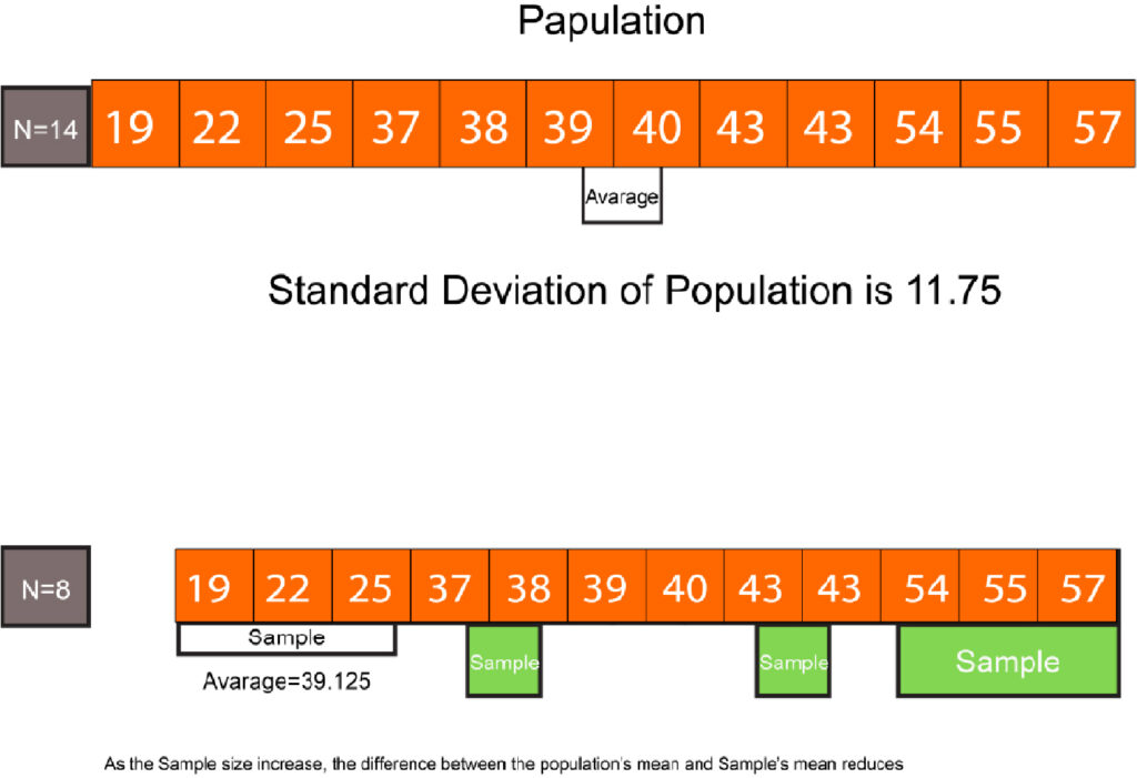
The formula for population variation/standard Deviation is recommended for formulating various statistical calculations if the population’s mean is known. The formula for Standard Variance or Sample Deviation is recommended if there is no population mean and is calculated using the average of the sample; however, when your sample is large enough(i.e., when you have lots in terms of numbers), then either formula to calculate the statistics will work as the difference is negligible as the standard error is reduced as the size of the sample. It is also possible to consider covering larger portions of the population. When our sample size is large, we’re more likely to be closer to the population’s mean, and the advantages of using N-1 as the denominator are reduced.

This is why Standard Deviation is among the most significant Measures of Variability available. In contrast to the Mean Absolute Deviation, it adheres to the mathematical principles and considers positive and negative values generated during the variance calculation. It can be utilized to analyze different algebraic concepts and for more detailed statistical analysis. However, it could be greatly dependent on the extreme values since the square of deviation greater than the average will result in higher output than one with less weight.
In this blog, there were a variety of ways by which we can better learn more about how data is distributed. Understanding the concepts behind Measures of Central Tendency and Measures of Variability will assist us in understanding the next blog post, Measures of Shapes, where the different shapes that data may take and the way these shapes assist us in describing the data are explored.
