Correlation coefficients can be among the most widely employed statistical tools that are employed when we need to find out if the two variables are connected to one another or not. They also allow us to determine the strength of this connection. There are many kinds of correlation coefficients, but one of the most well-known ones is called that of the Pearson Product-Moment Correlation (Pearson’s correlation or Pearson’s correlation) and is extensively utilized for linear regression. For this method of correlation, it is necessary for both variables to have numerical (continuous) variables.
Direction of Correlation Coefficients
The most fundamental and essential feature of coefficients is their direction. Two possible ways to the correction coefficient are either negative or positive.
Positive Correlation
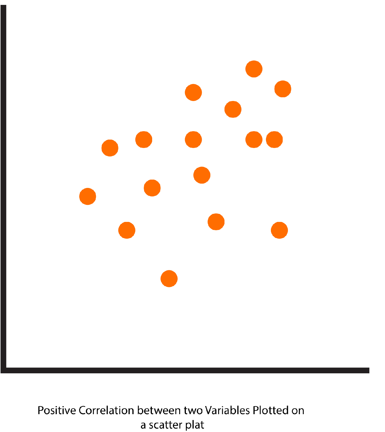
It is a sign that two variables are moving along the same line, and so for every increase for variable 1, there’s an increase in variable 2.
Negative Correlation
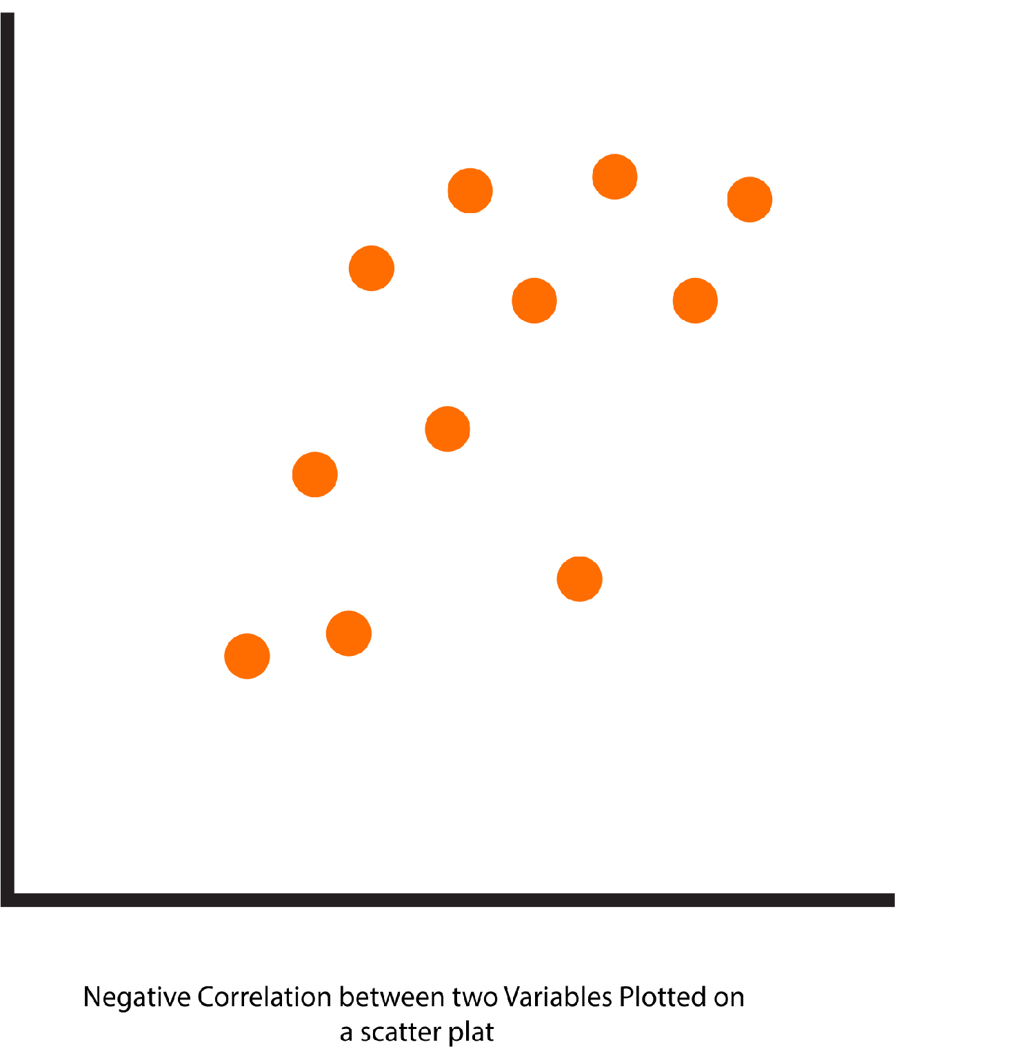
The two variables go in opposite directions, So for each increment for variable 1, there’s an increase in variable 2.
Magnitude of Correlation Coefficients
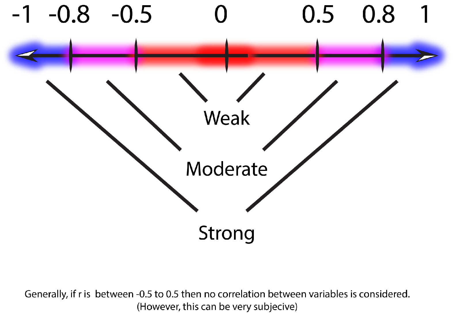
The correlation strength can be measured, ranging from -1.00 up to +1.00. When it comes to the Pearson coefficient, the letter ‘r is the symbol used to represent the coefficient. Its value is the measure of the direction of the correlation.
1 to 0

1 signifies a highly positive relationship. This means that for every increment in Variable 1, There is an equal growth in Variable 2. The positive correlation could range from 0 to 1.
R = 1. Perfect Positive Correlation
r = 0.8 Highly Strong Positive Correlation
r = 0.5 Moderate Positive Correlation
r = 0.3 Weak Positive Correlation
R = 0 – No Positive Correlation
If the r exceeds 0.5, then it is believed to be correlating; however, this can be extremely subjective.
-1 to 0
1 indicates a strong negative relationship. In other words, each time a unit increases in Variable 1, there’s an equal amount of reduction in Variable 2. The negative correlation could range between 0 and 1.
r = -1 – Perfect Negative Correlation
r = -0.8 Very Positive Negative Correlation
r = -0.5 Moderate Negative Correlation
r = -0.3 Weak Negative Correlation
R = 0 – Negative Correlation
0 (Zero)
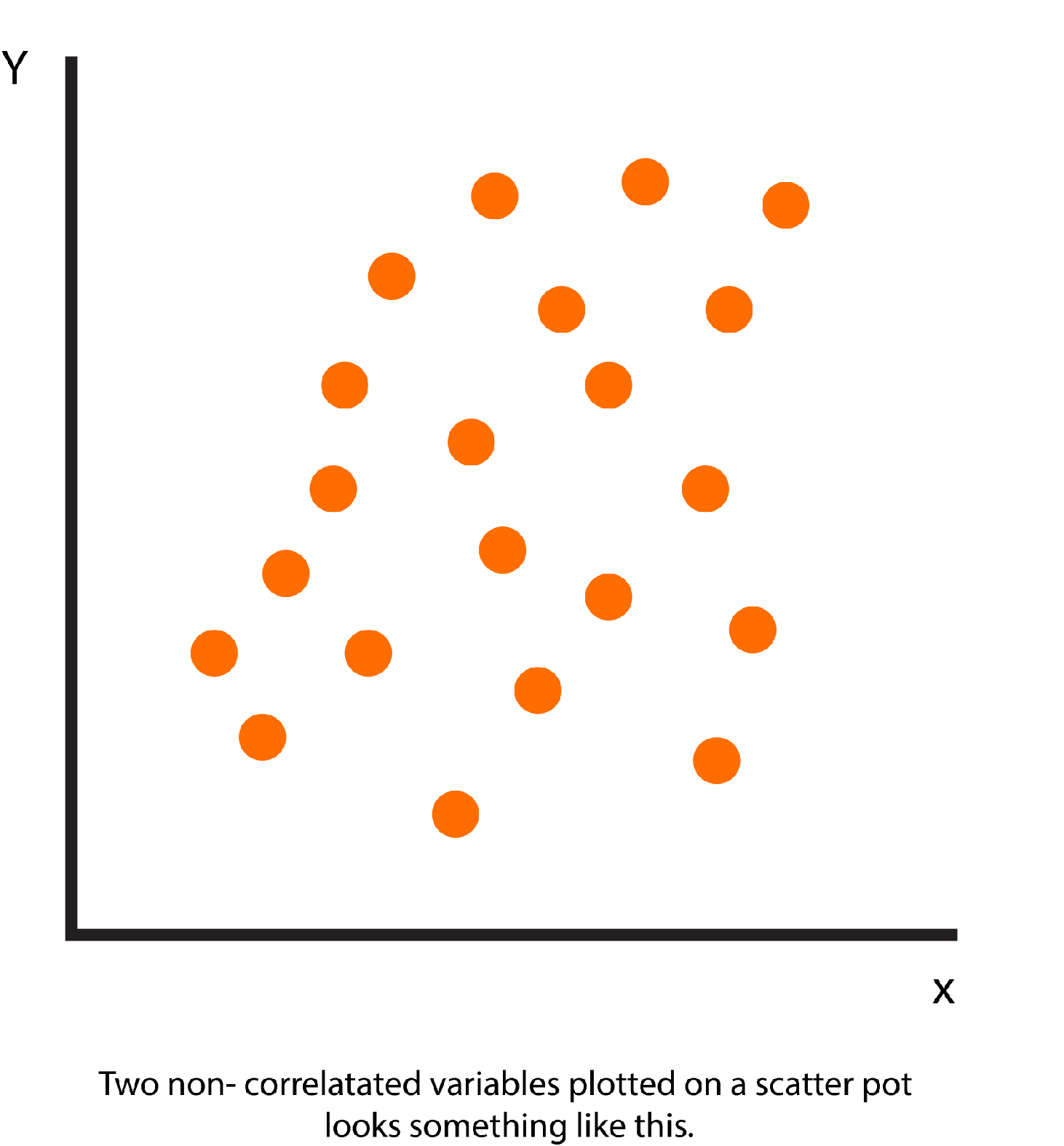
Zero represents that there is no relationship between the two variables. Also, for every increment in variable 1, there is occasionally be an undetermined change or decrease in variable 2. There is no evidence of any correlation.
Two non-correlated variables plotted on a scatter pot look something like this.
An example of no correlation could be the speed average of your vehicle and the number of wildfires that occur around the globe. The fact is that there could be (probably) no connection between them.

Calculation of Correlation Coefficients
There are various ways to determine correlation coefficients. In order to calculate the Person’s Correlation coefficient, the data needs to be standardized. The sum of the cross product between z scores on the two variables has to be determined, i.e., multiply every individual score on one variable by the score of the other variable, then take the total this and divide by the number of pair (N). The output is known as Covariance, but we will get the correlation coefficient if we standardize the covariance. The formula above makes it easy to standardize the variable before discovering a cross-product.
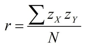
Positive and Negative Correlation coefficients are produced when an individual instance is scored lower than the mean value in variables 1 and 2. Their cross product would produce positive results (when two negative numbers will be multiplied and the result is positive). Similarly, if the score was positive for both these variables (above the average), the coefficient will also give positive results. This is the method that produces a positive coefficient. Suppose the case in question has a positive value for variable one (the value is higher than that of the median of the variable) and an opposite value for variable 2 (the value is below the mean variable 1). In that case, their cross product will produce a negative result (positive values multiplied by negative creates negative output). This is how we obtain a negative coefficient.
Determining Statistical Significance of Correlation Coefficients
To determine whether the amount of Correlation Coefficient can be considered statistically significant or not, the T distribution could be utilized. The formula used to calculate the t value is t = r-p/sr, with r being the coefficient of correlation between samples and p being the population correlation coefficient, and so is an estimate of standard deviation for the correlation coefficient for the sample. To avoid having to determine the standard error and then apply this as our denominator, an easy formula can be employed-
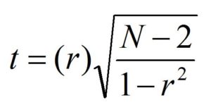
In this, the degree of freedom is N-2. Along with comparing the t value with the level of freedom. The significance of statistical statistics can be determined using the table of t.
The coefficient of determination (R2 /R-Square)
To determine if the value of the correlation coefficient indicates that there is a strong correlation between variables, the coefficient of determination may be utilized. The coefficient of Determination is also called R-Square (symbol “R2”). This term is frequently used, especially in linear regression, to evaluate the degree to which a model can explain and predict future results.
The coefficient of determination breaks down the issue to determine if the variance observed in variable 1 is connected with the variance observed in variable 2. This is because the coefficient of determination is used to describe how much variation of one variable is due to its connection with other variables, i.e., the extent to which our coefficient of correlation can be used in explaining the variability that is observed in one variable, based on the score of another variable. The coefficient of determination is explained in a manner that the moment two different variables become closely related but also share an amount of variance. Furthermore, a higher correlation means a higher proportion of variance that is shared between the two variables. The exact share (explained) variance can be determined by quadrupling the coefficient of correlation (r) that is provided with the Coefficient of Determination (r2)
The Limitations of Correlation coefficients
The issue of truncated range could occur when either or both of the variables at issue don’t show much variation in their distribution (due to the ceiling or floor effect). This is, for instance, when you’re trying to establish an association between the number of hours students spend studying and the marks earned by students. It is possible to find a situation where there is some variation in the variable 1-time that students study; however, there is hardly any variation in the variable 2 marks earned by students since every student scores very high (causing the ceiling effect).
The correlation coefficient is also incapable of determining by the 2 variables to determine which is the dependent variable and which one is the independent variable. Therefore, two variables can be linked, such as with a correlation coefficient of 0.6, but the same results can be obtained if the variables are swapped. When a 0.6 correlation is observed between eating junk food and obesity, then it can be said that the more junk food consumed, the greater the chance of becoming obese, but if the variables are changed, and the correlation is similar; however the result is ‘obesity leads to junk food.’ This does not make sense, so dependent and independent variables must be considered. The term ’cause’ as which was used previously, is of equal importance and should be utilized taking a variety of factors in mind, as correlation does not provide a reason for causality. Correlation is simply the term used to describe the average values of one variable that are related to the values of another variable or otherwise. Still, causation implies that the rise or decrease (variance) in the scores of one variable occurs because of (cause through or caused by) the variation in the other variable. One example is that there is a positive correlation between long days and happiness. However, this is only an observation and not proof of causality. Longer days cause people to feel content, and other factors could be at play; for example, longer days are during summer, and if the sample is from a non-tropical nation, the happiness can be attributed to summer and not due to longer days by itself. Therefore, correlation doesn’t give enough evidence to establish causal connections between two variables and to conclude that there exists causality between the two variables.
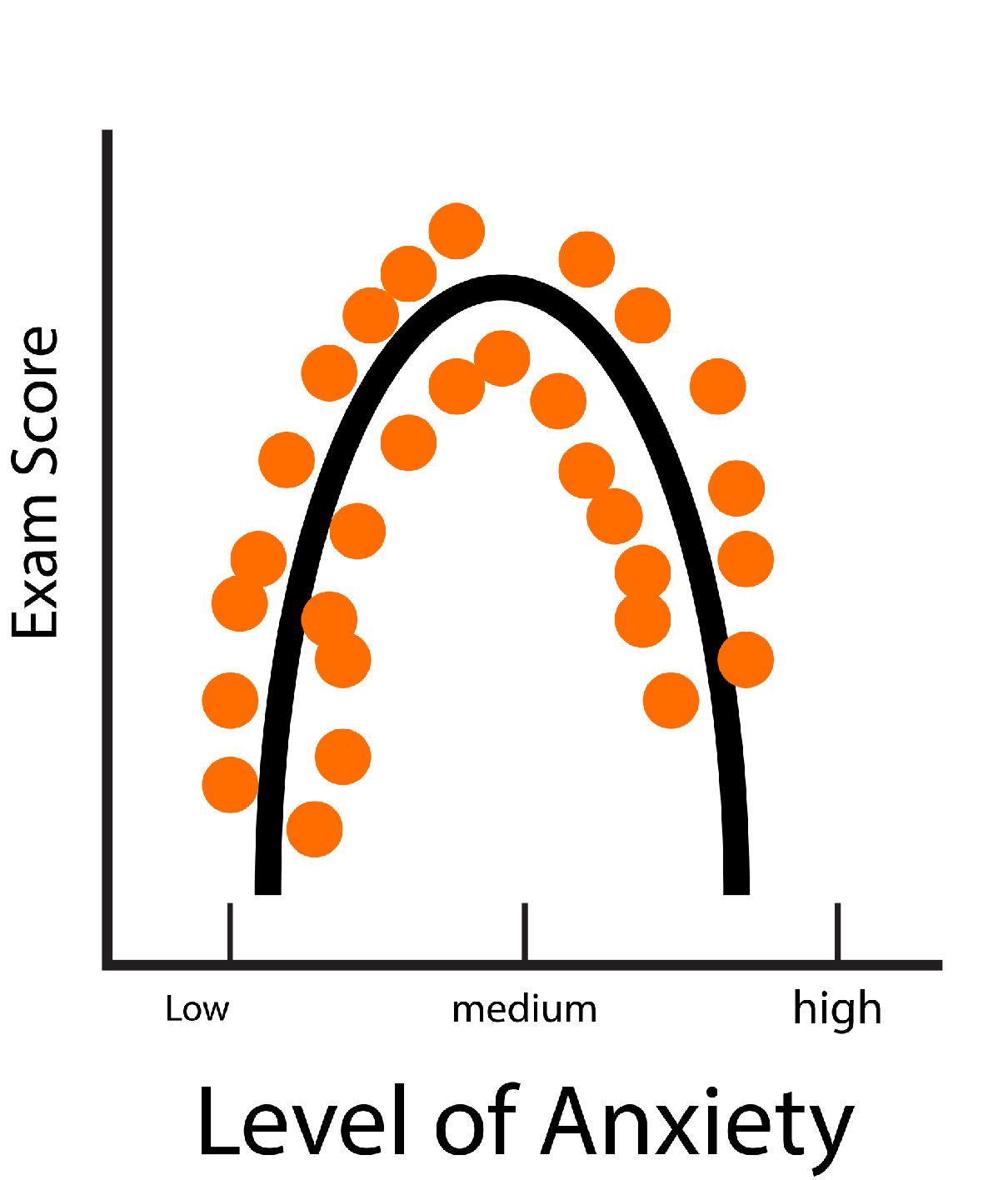
Pearson’s Correlation Coefficients are used to analyze the linear connection between variables. However, in the event that the relationship is not curvilinear, the correlation coefficient derived from this relationship is quite small, which indicates that there is not a relationship or even a weak relation between variables when an actual relationship could exist.
A good example of a Curvilinear relationship is anxiety and exam, wherein the rise in anxiety increases the scores attained by students, but if anxiety reaches some point, then the score begins to go downwards (negative relationship). In Curvilinear Relationships, One variable rises and vice versa. Variable, however, only to a certain level, following which, if one variable rises and the other decreases, the other one increases.
Other Types of Correlation
There are different types of correlation coefficients, like Point Biserial, that, unlike the Person’s coefficient, there is a continuous variable while the other variables are categorical two levels. For example, if you’re taking maths classes in college (Y/N) has a connection with the marks of the standardized aptitude test. Spearman’s Rho is a nonparametric test that is used to determine the degree of the connection between two variables. It can be employed for data that is recorded as ranks. And since ranks are an ordinal type, the Pearson Correlation Coefficient cannot be utilized. For instance, if the rank achieved in college is linked to the marks scored on the standardized aptitude test.
Pearson’s Correlation coefficient is useful in describing relationships among two factors. But, many other inferential statistics could be employed, for instance, tests using t-Tests or F-tests to determine the relationships between variables, even though the variables may not be numerical or contain multiple variables, etc.
EXPLORING F TESTS
F-test refers to any test that uses a test statistic that includes an F-distribution under an assumption of non-inference. In a sense, F-test is a generic term that covers all tests in statistical analysis which use F-distribution.
So far, the Z test and T tests are being discussed. Each test has its own distribution and formula for calculating its Z Value or the T Value. There are situations that cannot be conducted testing these tests. That’s when the F tests are beneficial. F tests employ F statistics, an equation of variances that is the sum of two. These F Tests use F Distribution. The F ratio is very beneficial and is utilized in a variety of tests (often employed to compare the statistical model). It is one of the well-known applications of this ratio is the comparison of two regression models to determine which one has statistical significance.
So, in contrast to the Z Test / T Test, in which the mean of two sets of data is compared in order to draw inferences for the purposes of the F Test, F statistic can be used to analyze two variances in order to determine whether the means from the different groups differ statistically from one another or not.
There are a variety of tests in which F statistic is utilized; however, the most popular F tests test is called the Analysis of Variance.
Analysis of Variance, more popularly known by its abbreviation ANOVA test, is an additional hypothesis test that differs from T and Z tests (whose calculation is based upon the distribution of data concepts of central tendencies, especially the concept of central tendency, particularly) and is built on variance. ANOVA tests allow us to decide whether or not to accept an unproven hypothesis. ANOVA can be used in cases in which Independent two-sample T-tests may be employed; however, F Test is more adaptable and efficient as compared to the test (ANOVA similar to Z or T-Test is utilized to determine whether the groups involved are similar or not, but as stated above in contrast to T and Z tests ANOVA utilizes variation to determine the differences in mean across the various groups.) In this case, it is the Null Hypothesis can be that there is no distinction between the groups, while the alternative Hypothesis is the opposite. For a better understanding of these situations, let’s look at some scenarios in which ANOVA is used.
- 100 people enrolled in an exercise program for weight loss are offered one of two types of diet (Diet Type 1 or Diet Type II), and you’re looking to determine which one is more beneficial over the other. (Here, we also have the option of using the Independent Two Sample test as the independent variable (Diet Type) includes two different levels (Diet Type 1 and Diet Type II)).
- Students from three schools prepare for their exams in history using strategies for memorizing that were developed by their school teachers. Which method is superior to one?
It is crucial to comprehend the meanings of ‘Dependent variables and Independent variables’ and ‘Groups/Levels.’ In the above-mentioned examples, the dependent variable is dependent on external factors. For instance, in the example, weight is the dependent variable. The independent variable is the kind of Diet, and the various subcategories that comprise the dependent variable are identified as levels or groups.
A variety of ANOVA variations can be used to test different kinds of data. Some of the most commonly used kinds of ANOVA are One Way ANOVA and Factorial ANOVA, Repeated Measures ANOVA, MANOVA, etc. A few of these kinds of ANOVA have been described below.
One Way ANOVA
One-way ANOVA can be used to evaluate the mean of two groups of the independent variable to determine if the groups are significantly different.
Factorial ANOVA
The concept is an evolution of One Way ANOVA, where groups of dependent variables can be compared to determine the extent to which they are statistically distinct from one another or not.
Repeated Measures ANOVA
Repeated Measures ANOVA analyzes groups with similar characteristics. In this case, ANOVA uses it to determine the variance in the mean of the dependent variable for more than two-time intervals.
