Outliers can cause issues in the functioning of different models and should be considered, especially in modeling algorithms like K Nearest Neighbour, which happens to be an algorithm that is based on distance. Different ways to deal with outliers are covered within outlier treatment. However, there is a machine learning technique called Anomaly Detection that could be used to recognize outliers. Outliers could be defined as observations that do not match the majority of data. Thus, different machine learning algorithms attempt to identify the observations that are different from other data, which could cause us to believe that they could be outliers. There are generally three types of Anomaly Detection settings: Supervised, Semi-supervised and Unsupervised. In this blog, Unsupervised Anomaly Detection will be addressed.
The Introduction of Anomalies
The most frequent situation is when one has to work with data that has less knowledge of the data. In this situation, identifying outliers and then determining if the data contains outliers is a major challenge. As discussed in the introduction of this section, finding anomalies under such a setup is very tough as the data at hand can be good, or it can, in all possibility, be bad and riddled with outliers/noise/anomalies. We can only assume that our data is populated with only a few outliers.
Unsupervised anomaly detection is based on the idea that anomalies that are not common are likely to be anomalies. To fully understand this, let us consider an example. Suppose we have a data set containing two features with 2000 samples. When it is plotted along the x – and y-axes, we can draw an image like this:
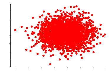
Looking at the graph, we will see that all the 2000 data points form an aggregation. We now know why the concept that a particular data point is uncommon will help us find the anomalies. If we attempt to determine the amount of data in this set and then estimate the density, we then score each of the 2000 data points based on the likelihood of seeing them within the dense area. So, from the data points, these are classified as anomalies that have very little chance of being observed, meaning they’re (figuratively speaking) removed from the cluster/dense region. It is just an estimate of the value of anomalies.
If we only look at this image, we will discern that some data points are in the category of an anomaly because they appear unusual and in contrast to most data.
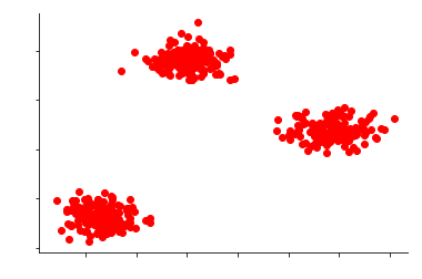
In many cases, the data are part of multiple clusters, and in such instances, our data might appear similar to
There are many kinds of unsupervised methods for detecting anomalies like Kernel Density Estimation one-class Support Vector Machines, Isolation Forests, Self Organising Maps, C Means (Fuzzy C Means), Local Outlier Factor, K Means UNC, Unsupervised Niche Clustering (UNC), etc. This blog will cover three techniques, such as Kernel Density Estimation and One-Class Support Vector Machines, as well as Isolation Forests, which were discussed. Rather than delve into the mathematical details of these methods, We will examine how these methods perform on the above data.
Kernel Density Estimation
Kernel Density is a non-parametric means to estimate densities. We can easily comprehend it using this method on our data. Let’s say our data is plotted on the x-axis, and the y-axis displays three clusters. We first determine the density for these three clusters using a fitting model to the kernel. The next step is to search for log probabilities that are single-valued values assigned to every data point. These log probabilities show the probability of a data point being observed in the density estimated in the fit process. It is then possible to eliminate data points that do not fall within the predicted density: the lower the log-likelihood, the more rare the sample. So, we are being able to identify the irregularities.
There are a variety of methods for measuring the density of data points. Histograms can be used; the completely non-parametric approach allows us to come into bins. The entire data point then fits into these bins, and those bins with the lowest number of points are categorized as anomalies. But, they are afflicted by an important issue with the increasing number of bins because when data is in high dimensions, these bins will grow exponentially. Another method that is commonly used involves Gaussian Mixture Models. It is a model commonly employed for Generative Unsupervised learning, i.e., Clustering, specifically expectations Maximization Clustering. A Gaussian distribution is explained in Section Basic Statistics. This is where Gaussian Mixture models are probabilistic models that are multi-modal distributed distributions. We present the data we have as a mix of Gaussians. Density estimation is often employed to aid in Anomaly Detection as it is more flexible to the data. These Density Estimation methods provide numbers that tell us how unlikely a data point is to fall within the density zone and then convert this information into anomaly scores.
Let’s first look at what we can see when we apply Kernel Density Estimation to our data.
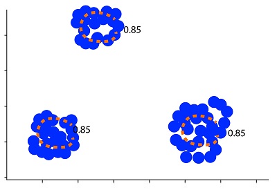
We employ the density function in which all data points inside the blue circles are within the high-density area and are regular observations. All data points beyond these circles are anomalies. In this case, we set the quantiles to 85 percent, which means that we’ve constructed the data in a manner that 15 percent of the data is in the circles. This is the most important parameter is required to be determined for Kernel Density Estimation, that is, an assumption that 15 percent of our data are contaminated. This means that we must establish an upper limit on the percentage of data that needs to be considered to be an anomaly.
If we alter the threshold to 95%, only 5 percent of the data could be considered an anomaly.
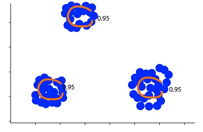
This method is extremely sensitive to threshold values. Additionally, an implicit parameter, in this case, will be Euclidean distance. Just like k, as the name implies, we require some kind of ground metric to measure the distances of various samples. As we’ve previously discussed, the methods that require the distance metric function have the same set of issues that must be resolved.
Additionally, this model isn’t effective in the case of data large in size like with all distance-based models. When the data is of extremely large dimensions, the space for data is nearly empty even though we have lots of data points, which makes estimating density difficult.
One-Class support vector machines
Support Vector Machines has been covered on its own blog. This blog will focus on One-Class Support Vector Machines that can be considered extensions to the previously mentioned Binary SVM, where one class is basically operating in an unsupervised setting. We will discuss the decision function that can be non-linear and based on kernels. The decision function, in this case, is a bit sparse in terms of the number of samples. This means that we only have a small number of samples that allow us to differentiate between the outer region and what’s inside. One Class SVM One Class SVM follows the similar concept of density regions, where the points that fall within a particular region are considered to be normal, while those outside are considered to be an anomaly. However, they’re better than Kernel Density as Kernel Density isn’t a good choice for very large dimensions, whereas One Class SVM estimates a decision function that works even in large dimensions. So, in contrast to Kernel Density which estimates density as well, One Class SVM is equipped with a decision function that informs you that if the amount of data points is too low, then it is regarded as anomalous or not.
The most fundamental and vital parameter we utilize can be the threshold, i.e., the portion of data we believe to be contaminated. When we limit our criteria to 50%, then 50% of our data is regarded as anomalies.
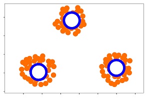
If we choose to take a higher number, for instance, 5 percent, then only 5% of our data is classified as an aberration.
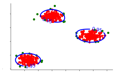
Another crucial parameter is gamma, which is an often used parameter in kernel-based SVMs. Gamma is understood as a bandwidth-related parameter of the kernel. If we apply only a small portion of gamma values, then we’ll have an extremely wide Gaussian kernel, which means we’ll be modeling our data in one large mode. But, in many instances, it is not an easy Gaussian distribution but a mixture of Gaussians. In this instance, we can observe that it is composed of several clusters of data that include a Gaussian cluster. Thus, we don’t use only one mode but an array of multi-modal distributions. So, a singular big mode isn’t required.
Therefore, we must boost the gamma to increase the kernel’s capacity to accommodate three data clusters.
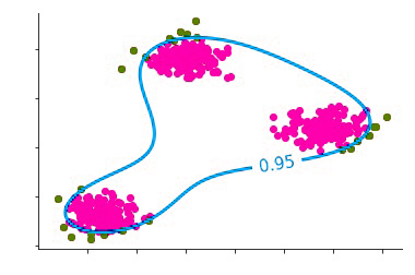
Suppose we do increase the gamma-value slightly too much. In that case, we’ll end up with a very complicated decision process as the kernel’s bandwidth will be such that it is unable to handle too many data clusters that might not even exist.
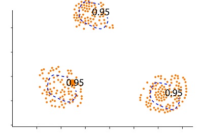
So, we don’t need to think about the proportion of data that can be considered to be anomalous but also the gamma factor that greatly influences the outcome.
Isolation Forest
The method for Anomaly Detection is built on trees. In the article on Decision Trees, we know that it’s an effective method in which space is divided by a variety of partitioning methods. The partitioning of data occurs through splitting across the axis direction. The technique can be used to separate specific data points. For instance, in the case of one feature, then all of these data points are located along the x-axis. Then, we can identify the data point distinct from the data points and divide the axis so much that the point from different data points lies on the opposite side of the division.

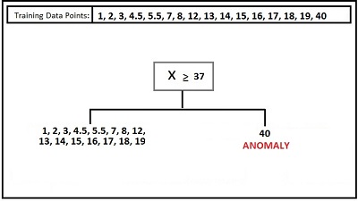
This is the way to identify the anomaly within only a few decisions, i.e., a few splits. This method lets us make a few random trees. We then select an unspecified feature and a random threshold. If the data point is located in a far-flung, scarce data space area, it can be separated by this random splitting. This is why we create random trees and then determine how many splits are required in order to separate the samples. If we determine the ideal depth, then the sample will be isolated in the leaf within some splits. The trees are constructed in a series of steps as we seek to determine the median amount of splits needed for separating a sample, and as a result, we add an even more stable process. Isolation Forest Isolation Forest uses this method and comes up with the values for different data points, which indicate the level of abnormality or anomaly.’
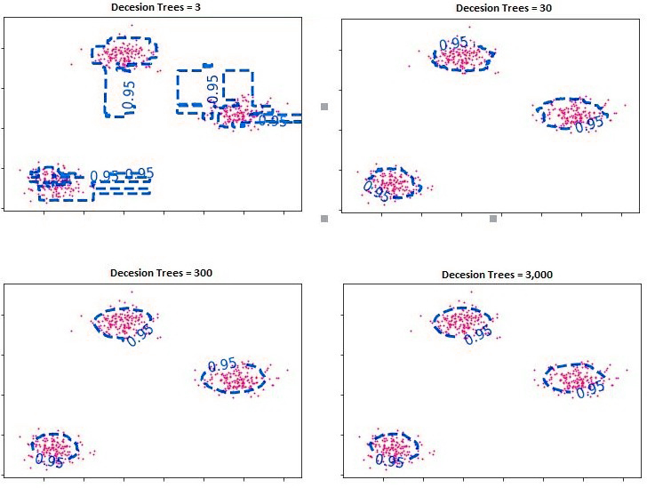
In addition to the quantity of data we wish to classify as anomalies, another important factor is the number of trees used to make decisions. If we use too little of a number, we create a decision boundary that is too complicated, so we should add a few trees to help regularize the decision process. By adding a larger number of trees, we can have more data to calculate averages from, which adds greater stability to the model. However, everything adheres to the principle of bias-variance. A low number of trees can make the data more complicated and less general. A high number of decision trees could cause oversimplification of the decision function, which causes the model to be unfit.
However, in this situation, when there are a lot of decision trees in the system, the problem isn’t about underfitting but rather the time and cost of computation, as after a certain amount of decision trees, an expansion of them won’t make a difference to the solution. It may not cause underfitting, but it will waste resources (time and other computation costs).
There are a variety of methods for the detection of outliers and their treatment. These are all discussed in the blog: The Outlier Method, which uses various statistical tools that can be utilized to find and treat outliers. The blog post analyzed much more advanced methods to identify outliers. Unsupervised models could be used to find outliers, and these outliers could be dealt with using the techniques discussed in Outlier Treatment.
