Factor Analysis is a classification method that operates within an unsupervised system. It helps to determine the commonalities between various aspects and then create groups of them, which it achieves by removing the highest common variance from all variables. The most popular use is that Factor Analysis is for Data/dimensionality Reduction, using it to assist in reducing the number of features by identifying variables strongly related to one another. In order to perform Factor Analysis, we require continuous variables (numerical and interval scaled) with sufficient sample size.
Factor Analysis is often difficult to comprehend in the absence of an illustration, which is why an example is provided to explain the method of factor analysis.
Introduction to an Example
There is a data set that has a dependent variable (Y_variable) is, “happiness,” it is a binary categorical value with two values: zero and one, which means “unhappy,” and 1, which means “happy.” There are 20 independent variables, and it is necessary to reduce this number of variables. If we know the process by which these 20 variables were developed. The fact is that the 20 variables were derived from four separate surveys, where each survey included five questions that gave an answer between 0 and 5 for each response.
(For instance, 5 out of five independent variables come to a single study Survey-A which contained five questions).
SURVEY – A
Q1: How is your pay?
Q2- How content are you with the work you do?
Do you enjoy your workplace?
Q4: How do you perceive your boss’s understanding?
Q5: Do you see an opportunity for growth in your job?
Latent Variable
Each of the questions above isn’t random, but they are part of a larger concept which is known in the term ‘ Value, and each of them is a seen factor as their values are determined, i.e., they are observed from the responses. The observed variables in this example represent a “value,” which is referred to as an “unobserved variable,” which is also known as a latent variable, and it is named in this way because they aren’t directly measured; however, they are rather spotted and interpreted by the variables that are observed. So, in this instance, it is easy to determine that there are four latent variables, each having five observed variables. However, the data needed to calculate this isn’t available in the real world. Statistical analysis is needed to determine the number of values that can be put together in a particular construct. Also, when there is the requirement for more than one type of construct, then what percentage of the values of one are different from those of the other, making each construction distinct? This type of statistical analysis is referred to informally as Factor Analysis.
In our current example in the above scenario, suppose we do not have any details about the fundamental construct and all the variables appear to be independent of us. Now, the various variables we observe need to identify similar patterns of responses associated with the latent variable. In our case, we will discover these types of constructs statistically through factor analysis in a variety of the steps listed below.
EFA and CFA
There are generally two types of factor analysis: Exploratory Factor Analysis (EFA) and Confirmatory Factor Analysis (CFA). EFA is the one that is being discussed in which variables that have a high correlation to one another are combined. This group is referred to as”factors.” After this factor has been created, it searches for other variables and then groups them into a different factor. The number of factors to be made depends on the analyst as well as the N (number of variables observed) amount of factors that could be made (i.e., one factor for every identified variable). The N number is determined by a variety of variables (discussed in the next blog).
CFA is employed to determine whether we know the latent variables and which ones belong to the same latent variable. For instance, we’ve got 10 variables, and five appear to have to do with education, such as: How important are formal studies for you? Are you happy with the present method of examination? The other set of variables appears to be related to sports, like how important are sports? How do you feel about the current conditions of training in sports? Etc. We can quickly conclude that there may be two latent variables. However, to prove this statistically, we need to conduct hypothesis testing, which is the area where CFA assists.
In this blog, we’ll focus on EFA because we don’t know what these hidden variables are or the number of them in the data.
Extraction and Factor Rotation
The fundamental idea behind the factor analysis concept is when we have all variables, we will have all the data that, in terms of statistics, means 100 percent variance. If we can reduce the number of variables but attempt to cover 70 to 80 percent of the data, that is, we attempt to capture 70-80 percent of the variance; thus, the aim is to reduce the number of variables while keeping much of the variation generated through the variables. To achieve this, we’re placing variables into groups known as factors. But, at first, we don’t know how many groups are going to be made, and in the majority of statistical software, it is a hit, and a test technique is employed. The rule of thumb is that every factor contains 4 variables. Therefore, you divide your total variables into either 4 or 5, and the result is the initial number of factors needed to perform factor analysis. In our instance, we will use 20 / 5 = 4. Therefore, we will perform the factor analysis using four factors. Factors Analysis employs a technique called Extraction to group all variables into four factors. This method first identifies the biggest group of variables that are highly related to one another. It then forms a group out of the variables. This group (factor) is the one that explains the majority of the variance among every variable that is analyzed. It then identifies the next set of highly related variables, and this factor is responsible for the second-highest variance in all variables, and the list goes on. In our case, we use an approach that has four factors, so we arrive at four factors.
The output appears to be similar to this:
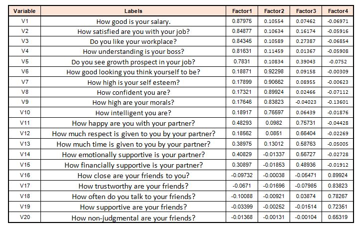
In this case, each row or analysis is loaded with a factor. The results of these factor loadings are very similar to correlation coefficients in that the higher number indicates that the variable significantly impacts the category (factor). The output is produced by extraction, but there are many ways by the extraction process, for example:
- Principal Component Analysis
- Maximum Likelihood
- Image factoring
A very widely employed method of extracting, which will be briefly discussed here, is Principal Component Analysis.
When performing Principal Component Analysis, the most variance is derived and then incorporated into the initial factor. When constructing the second factor, the variance caused by the initial factor gets eliminated. This is the process that is used for all factors. This method of extracting is so widespread that it’s the standard factor analysis method in most statistical programs. As we said earlier, the factors have to be distinct from one another, and to accomplish this, the variable’s area is turned, called the factor rotation. There are numerous methods to rotate the spaces. The most popular method of rotation used in Principal Component Analysis is VARIMAX, where we calculate the most variance by rotating the principal Axis. This type of rotation can also be referred to as orthogonal rotation. Other ways of rotating are available, for instance, PROMAX or Oblique Rotation, in which the assumption that factors are orthogonal is removed, creating factors that are linked to one another.
Both of these strategies for rotation are essential and should be utilized. Still, PROMAX is usually considered superior in real life, in which the factors are moderately dependent on each other and won’t be quite as different as in VARIMAX; however, VARIMAX is easy to evaluate, understand and, therefore, offer its own set of advantages. Other strategies for rotation include Quartiax, EQUAMAX, etc. The general rule is that VARIMAX can follow PCA. The former builds latent variables, while the latter makes the factors distinct.
At the very end of it all, it is important to keep in mind that the purpose of all Rotational Strategies will be to get clear patterns of loading that are easy to identify and differentiate the higher loadings from the less loaded for each aspect. (see in the next image)
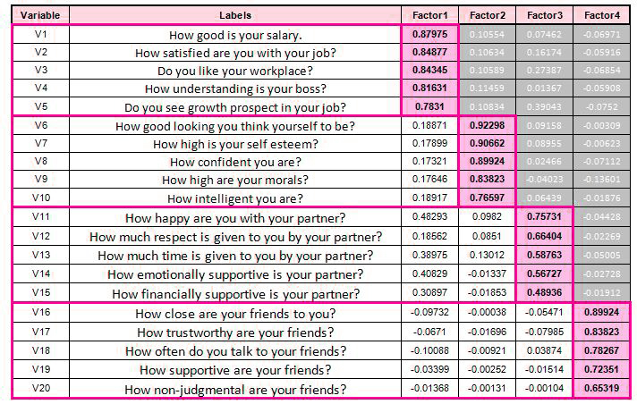
If this factor rotation method is not utilized, we would be left with multiple factors that would all be based on the same variation found in the connected variables. As a result, they cannot attain the truly diverse, less closely linked variables.
PCA v/s PCA
The blog post on Principal Component Analysis discussed its usage as a method to reduce dimensionality. However, for Factor Analysis, which is not a feature reduction technique, We are using principal components here. It can be tough to differentiate between these two PCA, particularly when the majority of the statistical programs use Principal Component as the default method of extraction used for Factor Analysis. To be specific, it is important to know that Principal Component Analysis as discussed in the earlier blog Principal Component Analysis discussed in the previous blog can be described as an autonomous analytical approach that is the approach to reducing features commonly employed when variables are heavily connected, which is reduced to a lower quantity of fundamental components that make up the majority of the variation of the variables. Principal Component Analysis here can be thought of as a mathematical transformation. However, this blog uses Principal Component Analysis to extract factors as a method, i.e., an instrument to create latent factors. In this case, we estimate factors and randomly select the variables for the purpose of modeling in the future. This is where factor Analysis functions more as a technique used in statistics to categorize variables and select those of interest by maximizing their variance. Therefore, two distinct models can be employed to reduce feature size. PCA is orthogonal, meaning that the components are linear combinations in which the variance of all components is maximized. In FA (Factor Analysis), PCA is used to determine factors. However, there are components of linear combination where the proportion of shared variance is maximized.
Determining Number of Factors
As mentioned at the start, Factor Analysis will require some trial and error before we arrive at the most effective solution. We have decided to conduct EFA, assuming we know nothing about the fundamental concepts. We began the exploratory factor analysis process by choosing a selection of factors using the thumb rule of the number of variables divided by five (considering that each factor has five variables). Then we chose the extraction method to produce the latent variable. We chose PCA and, for instance, Orthogonal Factor Rotation to distinguish the factors from one another. The information entered into the statistical software creates a Table of Communalities, which is used to decide the number of factors that should be utilized.
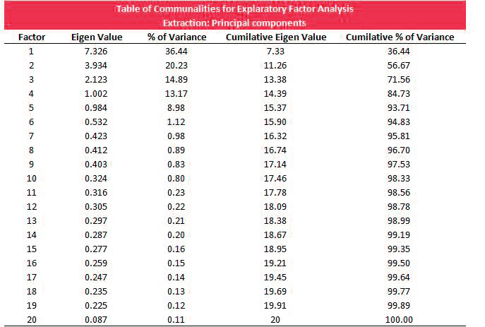
Understanding the Table of Communalities is very crucial to be able to determine the number of factors. This is the first column for the number of factors. As we mentioned, there are numerous factors, as many variables, we can observe. In the second column, Eigen Values are listed. The third column is constructed from Eigenvalues alone, which shows the % of the variance. We can observe that Factor 1 is the one with the most variance. This means that we’ve achieved the maximum variance (36 percent) in the information on this factor. The second factor is responsible for about 20% variance, and the percentage diminishes with the factors. The second column provides the cumulative Eigenvalue, while the final column shows the percent of the variance, which is explained by each factor.
The first step is to comprehend these columns by observing them intuitively. The column on factors is about how many factors account for the variation. If we select 1 factor, i.e., the minimal amount of factor, it will give us an amount of factor in which all variables are combined. If we select factors from this factor, we could reduce the multicollinearity, but we’ll have to combine variables that are fundamentally different forcefully. In addition, we’ll be losing a significant amount of information since the overall variation explained by this factor is just 36 percent. If we increase the number of variables by 1, we increase the likelihood of multicollinearity but also the variance that is explained. In addition, we release the variables that were forcefully grouping them. If we continue moving to increase the number of factors, those variables which are supposed to be together will begin to split, and deciding which variables have an equal basis will become difficult. This will eventually lead to multicollinearity, which will destroy why factor analysis was done, i.e., feature reduction. Please note how the final factor has the highest total variance, i.e. when we include all the factors, we will not lose any data. This means that we can utilize Eigenvalue as a synonym for multicollinearity as well as variance as an alternative for data that has been captured. We need to consider the pros and cons to ensure that we strike an equilibrium between multicollinearity and the data that is captured.
The Kaiser criteria
In accordance with this measure, it is only possible to keep the number of factors for which the Eigenvalue is greater. The concept behind it is this: if a factor is responsible for less than 10 percent of the variation, it might not be as beneficial.
In practice, the ideal Eigenvalue will be taken to be one that is less than 1. This is to limit the impact of multicollinearity.
Scree Plot
You can also determine the number of variables by plotting the Eigenvalues of the variables on a straight line graph. The method involves determining the point at which the smooth decrease of Eigen values is leveled off, and the aspects around that elbow can be considered.
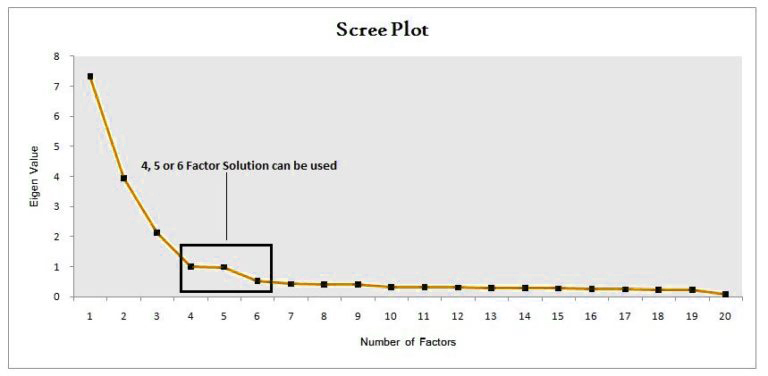
In this example, a 5-factor solution is possible; however, the use of hit and test with different factors is required in real life.
Selecting Variables
The final step involves selecting the variables that are relevant to each factor. In this step, we will select the variables with the most factor load for the particular factor and choose the pertinent variables. This is a subjective process, and the variables chosen for each factor are based on a variety of factors, including the business environment, demand from clients, etc.
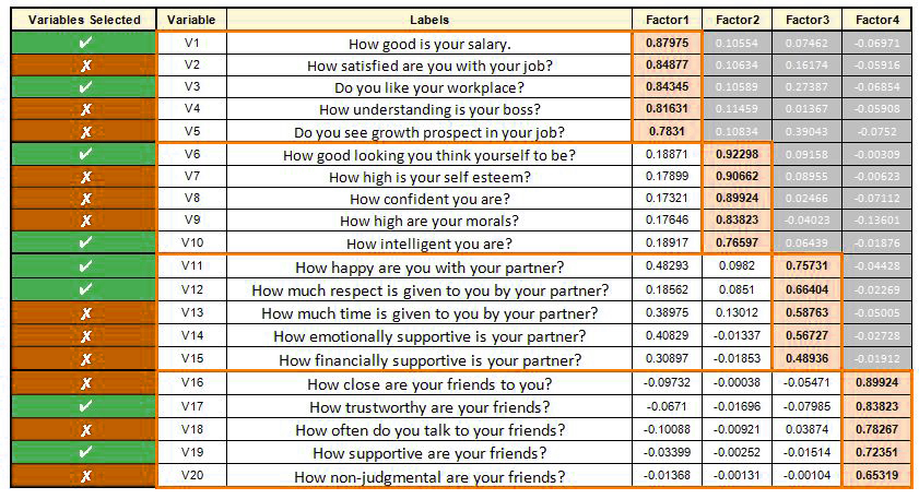
In this, we can see that the employment-related factor plays an important role. It was also identified as the primary factor causing approximately 36 percent of the variation, with factors such as the amount of money earned and satisfaction with the job having high loading. Growth prospects have a relatively low loading, but the variables we choose are subjective and depend on various factors.
So, we’re capable of putting all our variables into “factors” that share a common concept or background to them.

It is an effective method of classification. However, we can utilize this method to select variables by grouping them into closely related variables with significance to them. This technique requires a little to and from but is very useful when forced to limit to a minimum the number of variables we have and make some uninformed choices.
