Hierarchical Clustering, a Hard Clustering Method, is unlike K-means (Flat Clustering Methods). Still, we arrange the data in an order where there is one large cluster at the top, and at the bottom, there are as many clusters of observations as the dataset has.
Agglomerative v/s Divisive Clustering
There are many methods to create a hierarchy. However, the most well-known hierarchical clustering algorithms are:
- Agglomerative Hierarchical Closing Algorithms
- Divisive Hierarchical Clustering Algorithm for (DIANA).
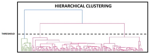
Below is a Dendrogram that is used to show a Hierarchical Trees of Clusters diagram. This diagram can help you to understand the difference between Agglomerative vs. Divisive clustering.

Agglomerative Hierarchical Clustering Algorithms: This top-down approach assigns different clusters for each observation. Then, based on similarities, we consolidate/merge the clusters until we have one.
Divisive hierarchical Clustering Algorithm (DIANA): Divisive analysis Clustering (DIANA) is the opposite of the Agglomerative approach. In this method, all observations are considered as one cluster. Then, we divide the one-large cluster into smaller ones. These clusters can be further divided until there is one cluster for every observation.
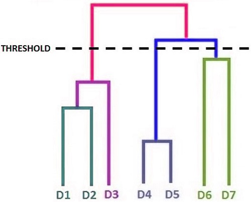
Each method uses a threshold to determine the number of clusters. Too high a threshold can result in clusters with more generalized meanings. However, the threshold that is too low can result in clusters that are too small to be meaningful. This threshold can be viewed as a cutoff on our dendrogram. The basis of the threshold could be dissimilarity.
Types and Links
As we have already mentioned, both methods require that the clusters be similar (agglomerative or dissimilar) to each other. This is done by calculating the distance between the clusters. There are several ways to calculate distance: Single Linkage, Complete linkage, and Average Linkage.
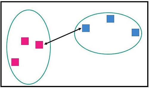
Single linkage (Nearest Neighbour).
We can cluster using a single linkage by finding the nearest cluster by computing the shortest distance between them. We use the nearest data points to determine the distance between the two clusters.
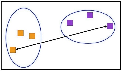
Complete Linkage (Farthest Neighbour).
Single Linkage is reversed. We consider the two nearest points of the two clusters. We use the greatest distance between the clusters to determine the proximity between them.
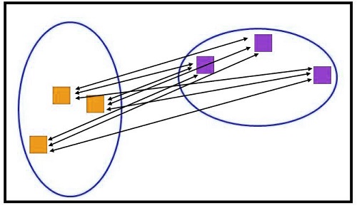
Average Linkage
Also called the Unweighted Pair Group Method, we use the average distance to calculate the average distance. We calculate the average distance between any data point in a cluster and all the data points in another cluster.
Other methods, like the Centroid Method, can also be used to determine the distance between the clusters. This uses the center points in the cluster. Ward’s Method, which minimizes squared euclidean variance (minimum variation), is another well-known method. The error sum of squares based on all the observations from the two clusters can be used to determine the proximity between them.
We’ve already covered Agglomerative and Divisive types of clustering. Because both methods are identical, we will only discuss one of them.
We will explore Agglomerative clustering by using Single-, Complete, and Average linkage methods.
Agglomerative Hierarchical Clustering
It is possible to take a dataset and use the single-linkage method to determine distances between the clusters in order to understand how agglomerative clumping works. For example, we have a dataset with two features, X or Y.
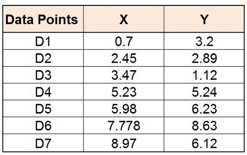
This graph will be generated when the data points have been plotted on the coordinates x/y.
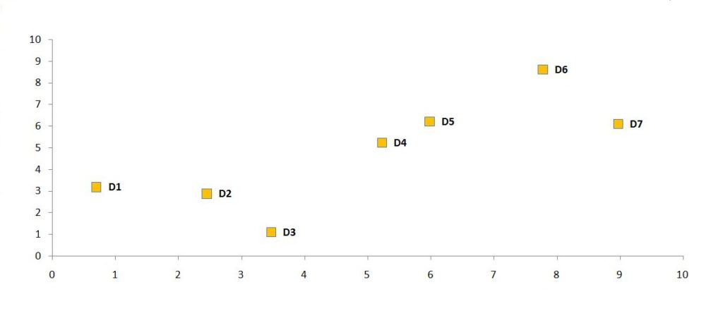
Hierarchical Agglomerative Clustering requires that you have as many observations as possible in your dataset. In our case, this is 7. We currently have seven clusters. We now want to continue consolidating data points to form clusters and to have one eventually.
Steps for Agglomerative Hierarchical clustering
Step 1
The first step is to create what’s known as a Distance Matrix. We calculate the distance from each observation in the dataset to the other. This example uses the Euclidean Distance distance metric.
The formula to calculate Euclidean distances is:

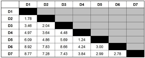
The formula above calculates the euclidean distance of each observation relative to all the others and gives us the table below.
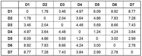
If you check this closely, you will notice that the distances between the upper and lower fold of the distance matrix are the same. You will also explore that there is a diagonal line of 0s. When we look at the distance between D1-D1, we see that there is 0 distance. From D2-D2, we get the same distance. Thus, the distance to D1-D1 is nil.
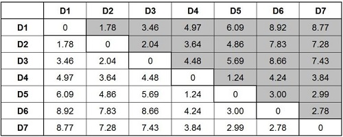
We have removed duplicates and 0 values to simplify things to create a simplified distance table.
Step 2
Agglomerative clustering, as mentioned at the start of this post, is a top-down approach. We merge observations together based upon their similarity (minimum difference). We examine the table to find the data points closest to one another.
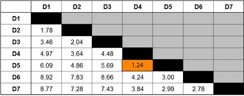
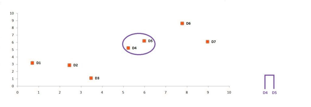
We find the minimum value in our table at 1.24. It is the distance between D4 (or D5). D4 is the nearest data point in the dataset, while D5 is the farthest. We can then combine these data points to create a group. Now we can visualize the cluster on the graph and create a dendrogram.
Step 3
Here is where we introduce the linkage method. We need to update our distance matrix by recalculating distances with respect to the newly formed group.
We need to use the single linkage method to calculate D1’s distance to D4 and D5. If you use the single linkage approach, we will look at the distances between D1 and D4 and D1 to D5 and choose the minimum distance that is between D1 and D4, D5.
When we look at the distance matrix, we can see that D1 offers two options: 6.09 (Distance from D1 to D5) and 4.97 (Distance from D1 to D4).

Because we’re using a single linkage, the minimum distance is chosen. We, therefore, choose 4.97 to be the distance between D1 & D4 and D5 and use it as such. If we had used complete linkage, the maximum value would have been selected as the distance between the D1 and D4, which would have meant 6.09. If Average Linkage were used, then the average distance between these two distances would be used. The distance between D1 (D4) and D4 (D5) would be 5.53 (4.97 + 6.99 / 2)
This example will create clusters only using a single linkage technique. The updated distance matrix can be found after we have recalculated the distances.
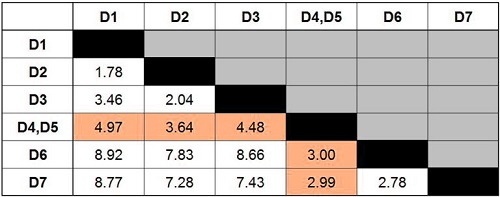
Notice that there is no column or row for D4 or D5 anymore. Instead, we have D4, D5, and D5 in a new row. Highlighted in yellow are the new distances.
Step 4
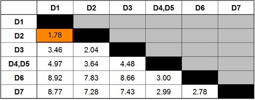
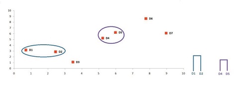
We will just repeat Steps 2 and 3 until we reach one cluster. We look again for the minimum value, which is 1.78. This means that the new cluster is possible by merging D1 and D2.
This cluster is now visible on the graph. We then update the dendrogram.
Step 5
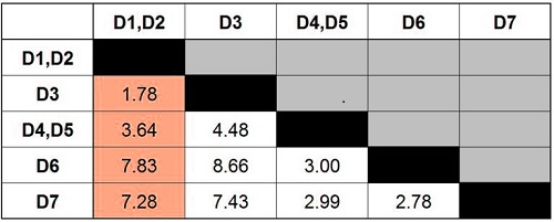
We repeat steps 3 and 4 to calculate the distance for clusters D1 and D2 once more. This time, we came up with this updated distance matrix.
Step 6
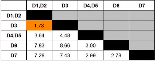
The minimum value in our distance matrix is found by repeating the steps from step 2. The minimum value of 1.78 indicates that D3 must be merged with D1 and D2.
We visualize the new cluster on the graph, and then we update the dendrogram.
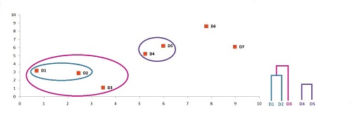
Step 7
Update distance matrix using Single Link Method
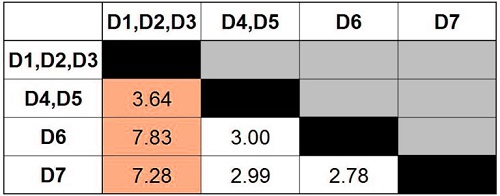
Step 8
Find the minimum distance in the matrix.
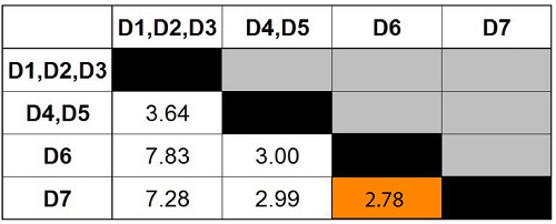
Take the data points and combine them to create a new cluster.
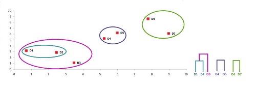
Step 9
Single Link Method to Update Distance Matrix
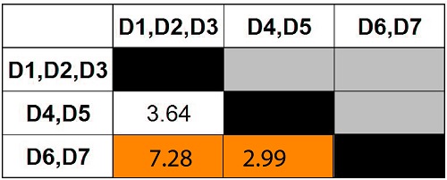
Step 10
Find the minimum distance among the clusters of the matrix.
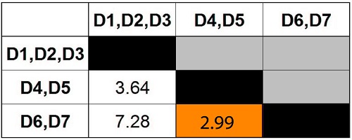
Combine the clusters to create another.
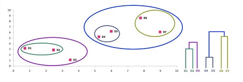
Step 11
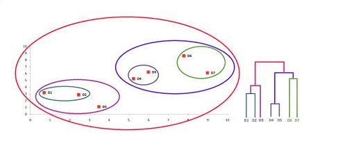
Given that we only have two clusters left, we can merge them.
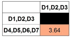
Finally, we have a single cluster.
Step 12
The thresholds can be used to create a variety of clusters that are meaningful to you. We can see three clusters that make sense if we examine the graph. The first is one where we combine the data points from the bottom left, the second is when we consolidate the data points from the middle, and the third is when we merge the data points from the upper right. This threshold can be visualized on the dendrogram. It will give us the three-cluster solution.
Merits & Demerits of Hierarchical clustering
Hierarchical Clustering is a great way to cluster because it’s easy to understand and apply without having to have a certain number of clusters. It is also easy to visualize and helps to make clusters understandable visually by using dendrograms.
However, hierarchical Clustering is sensitive for noise/outliers. Standardization is also required as distance metrics such as Euclidean distance, which require data on the same scale as the other distance metrics are used. To provide meaningful results, the data must be consistent. It is also very complicated, with the operation complexity being O (m 2log m), where m refers to the number of observations.
Dendrogram can be used to visualize clusters in hierarchical clustering. However, it is sometimes difficult to find the right number of clusters by using a dendrogram. You can either set a number of clusters that you want to be included in the hierarchical algorithm, or we can stop it once it has reached the desired number. We are now back to k-means clustering. Here we needed to know exactly how many clusters were to be found. The other way to find the right amount of clusters is to use cohesion. This indicates their goodness. Hierarchical clustering is a method that allows you to stop creating clusters if the value of cohesion in the clusters becomes too low. By doing this, you can get the right number. There are several ways to define cohesion. One way is to set the cluster’s radius so that the new clusters are less or more than the predetermined size. The algorithm will then stop creating clusters. You can also calculate the radius, which is the distance between a cluster’s centroid and its edge. The density-based approach is another way to go. This is where, instead of setting a threshold value for the radius or diameter of the clusters, we set the minimum number that should be in each cluster. If the algorithm fails to create clusters with these numbers, it will stop creating them.
Hierarchical Clustering has many advantages and disadvantages, but it is still a popular method of clustering. This is due to its visual approach and ease of understanding.
