In this blog post, an additional inferential statistic will be discussed, which is Chi-square. But, before we dive into the specifics of chi-square, it is essential to comprehend why chi-square differs from other tests previously discussed, such as the T-Tests or the F-Tests. To perform, it is important to be aware of the differences between Parametric and non-parametric tests.
Parametric and Non-Parametric Statistics
Parametric Statics

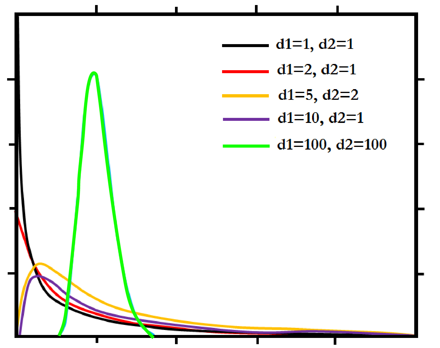
Parametric statistics can be used to draw inferences about the population parameters, i.e., in the past, we’ve drawn randomly representative samples of the population. By doing the statistical test on those samples, generalizations or inferences regarding the population could be made. Therefore, we employ statistical samples to calculate population parameters, also known as Parametric Statistics. In the past, we’ve utilized parametric statistics to determine the means and the differences between means of groups, and we have utilized a variety of parametric tests like F Tests and t-Tests, for instance. In all cases, we could draw inferences from the foundation of Null Hypothesis significance testing. Also, in all the tests we used, there was a specific sampling distribution, like T Distributions or F Distributions. Each of these was a particular group of distributions, where each family of distribution is selected according to the degrees of freedom dependent on the size of the sample.
T Family of T Distributions (Here, the distributions depend on the degrees of freedom where degrees of freedom is a function of the sample size) (This is Image Tagline)
F Family of Distributions (for ANOVA) (Here, the distribution depends upon the degrees of freedom which is a function of the number of subjects in the group and the number of groups we are comparing)
The inferences made regarding the general population is based upon the distribution of samples that are based on many assumptions (such as the homogeneity-of-variance as an assumption in ANOVA and Independent Test of t) and, if assumptions aren’t true and cannot be changed (if assumptions aren’t true there are a few tweaks or ‘fixes’ may be made, such as applying a limited error term, or changing the degree of freedom to ensure that parametric statistics could be employed) The parametric statistics must be eliminated and a non-parametric approach to be employed.
Non-Parametric Statics
Non-Parametric Statics doesn’t consider that the individuals in their sample possess any specific characteristic (such as being evenly distributed or having the same relationship between predictors as well as the result). It is worth noting that there are non Parametric tests for all types of parametric tests examined so far (Correlation, Z Test, t-Test, and ANOVA), and it is possible to employ non-parametric methods if needed.
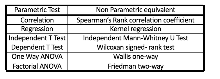

Some Non-Parametric equivalent of Parametric Tests (This is Image Tagline)
Some of the prominent differences between parametric and non-parametric statistics (This is Image Tagline)
Therefore, when populations are biased, or the assumption needed for the operation of parametric statistics is not met, non Parametric tests are very useful since they are simple to comprehend and no assumptions can be made regarding the distribution of the population. Furthermore, Non-Parametric Statistics employs medians, which are more effective when data is biased (Refer Measures of Central Tendency). Additionally, non-parametric tests are efficient when the test sample isn’t sufficient. But it is necessary to note that certain Non Parametric tests can only deal with ordinal or nominal scaled data. They are not as effective as parametric tests.
Learning Chi-Square by providing an example
This blog discusses the chi-Square test among the top effective tests that are not parametric—Chi-Square test.
The Chi-square test employs two categorical variables (or nominally scaled variables). It is a non-parametric test since it does not make any assumptions regarding the sample’s characteristics when conducting it. It is also called as the Goodness of Fit test. The Goodness of Fit test can be used to determine if any given distribution is matched to the sample properly or not (in terms of whether the data from the sample is comparable to the information you’d imagine to see in the real population as well or otherwise) and is utilized in statistical tests such as Chi-Square and Shipiro-Wilk tests, as well as Kolmogorov-Smirnov and so on.
A good example is useful to help you understand how the Chi-Square functions.
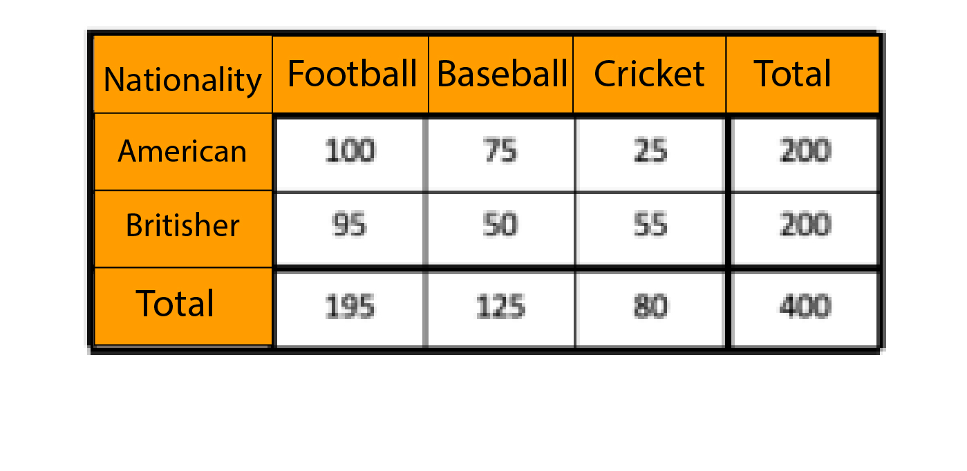
Two categorical variables are available one is called the Country of Origin, which has two levels, namely Britisher as well as American. The second categorical factor refers to what we call the Type of Sports which has three levels: Soccer (Soccer), Baseball, and Cricket. There is a center for coaching in which training for all these sports is offered. We have a sample data set in which the number of Britishers and Americans enrolled in different sports is recorded. We must determine the relationship between the Country in which an individual is from and the sport that he selects.
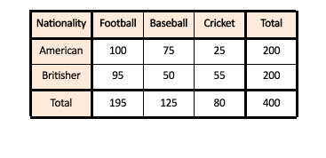
The Observed Frequencies Table
Chi-square is a method of working by comparing data we’ve collected (The observed Frequencies Table) against the frequencies that we would have predicted (Expected Frequencies table). The Expected Frequency table will include values we’d anticipate in each cell purely by chance. The ‘expected values can be calculated by simply using the group’s total count, e.g., we are trying to determine the expected value of Americans who are likely to enroll in the sport of football. We will consider the total number of Americans (which is, in our case, 200) and divided by the total number of people in the sample (which in our case will be 400) and multiply this figure by the total count for the other group which, in our instance, will be 195 (the number of players that are enrolled in the game of Football). Therefore, if we need to determine the expected value of the number of Americans enrolled in Football, We will calculate the total number of Americans and the total number of players taking part in Football along with the total number of people in our sample. We then take these figures to determine an expected amount. The equation for that particular column would be:


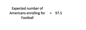
In the same way, we compute the expected values for each combination, and we end up with an Expected Frequencies table.
Expected Frequencies table
It will sound interesting to look at the relationship between our Observed Frequencies Table and the Expected Frequencies Table.

It is fascinating to observe that the results of Americans, as well as Britishers in each of the sports, are the same expected value. This is because the size of the sample groups in the variable ‘Nationality is identical. Because of this identical size, we are able to assume the same equal amount of Americans and Britishers for each sport. We can see that the significant difference between the measured and anticipated values is in Baseball, Cricket, and Football, while for Football, there isn’t much variation between the expected values and the observed values. The Expected Frequencies Table is also known as a Contingency Table. It is a table that uses chi-square; the test we’re performing, in this case, is the chi-square test of independence. We can determine whether the amount of cases (or frequencies) within every class (group or level) of each variable is dependent on (contingent on) the level or category (group or degree) of the other variable or not. The main thing we want to test in this case is whether the number of players who sign up for Cricket depends on your nationality, i.e., being a Brit or not.
Now is the time for hypothesis testing, whereby we will be able to determine if the variance in frequencies is statistically significant or not. Similar to what we found with t-values for t-Test along with F value in the case of F Test, we have a Chi-square measurement statistical value (Kh2), and the formula used to calculate it is explained below.
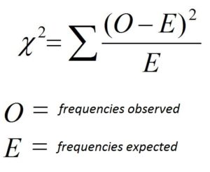

Before we look into the Chi-square table, we need to look at what degrees of freedom are (just the way we did before investigating the t-Table as well as the F Table) as the Chi-square distribution is determined by the degree of freedom (the method in which t, as well as F tables, are based on their freedom degrees)
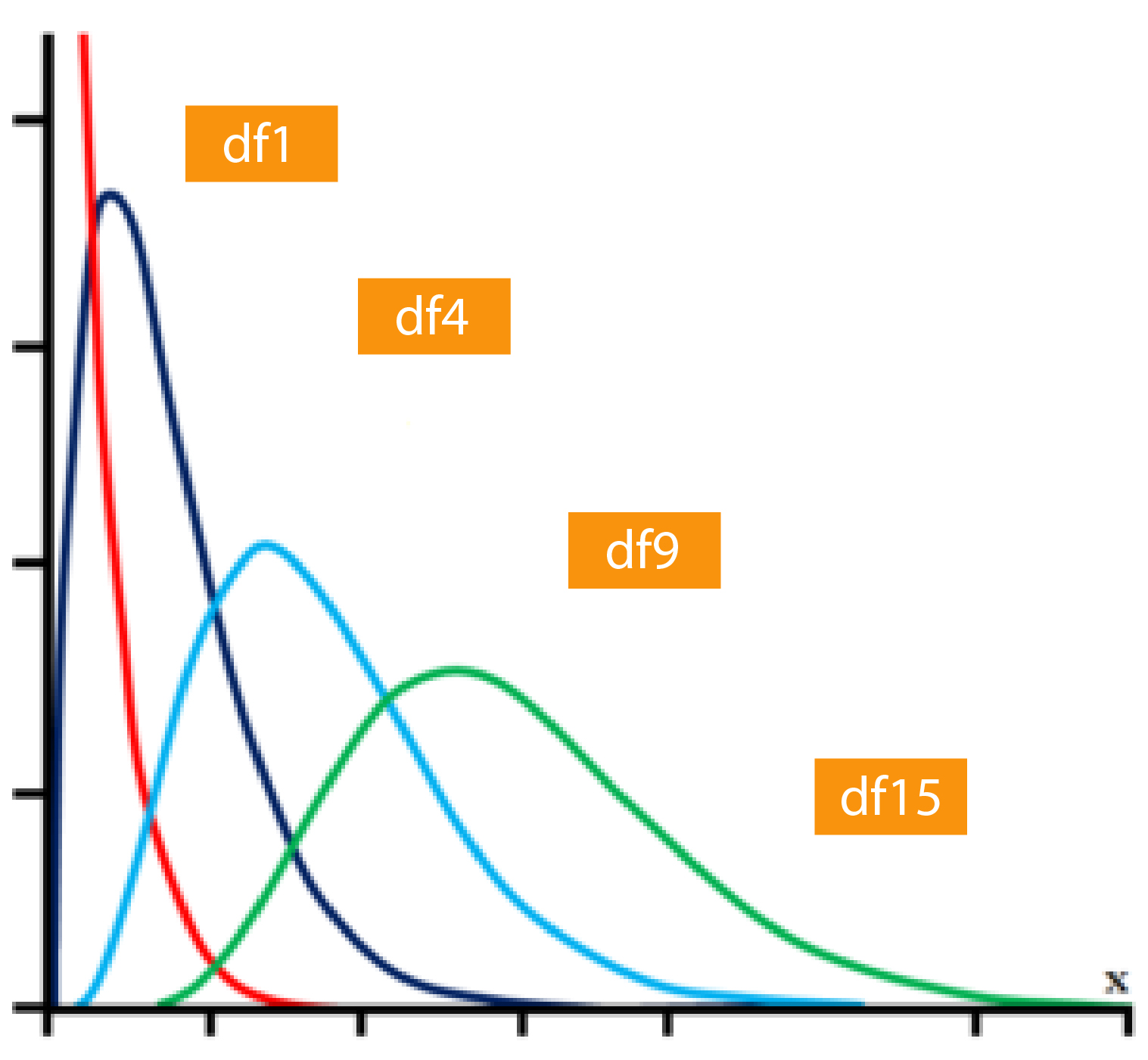
Chi-Square family of distributions
The degree of freedom refers to the number of groups. We have two categorical variables, two groups are present (Nationality: American and Britisher), and the second has three groups (Sports such as Baseball, Football, and Cricket). Simply put, the degree of freedom is the number of rows of the contingency table minus 1 multiplied by the number of columns of the contingency table minus 1. In this instance, this degree would be
df = (2-1) (3-1)
df = (1) (2)
df = 2
Now, let’s have a look at our chi-square table.
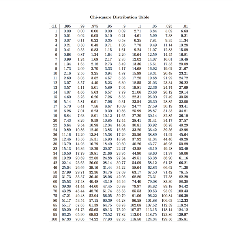
Suppose we take an alpha value of 0.05, which is the critical Kh2 number of 5.99. And since our Kh2 value is greater than the critical number, we conclude that our p-value is lower than 0.05, and therefore we are able to reject that hypothesis. Null Hypothesis, and also, as usual, the Null Hypothesis affirms that there is no connection among the variables. Both variables are independent, and the other hypothesis claims that the opposite is true. Therefore, we can conclude that an individual’s nationality played an important role in his choice of sports.
Chi-square is among the most significant and well-known non-parametric tests. It is employed when we need to evaluate the categorical characteristics of two variables. After acquiring the basics of statistics, we can begin to make our data ready to model.
