In n our previous post, concepts like the central Limit Theorem were discussed to give an understanding of how samples may take on a similar shape to the distribution of population and how the mean of a sample can be in line with the average of the population. Based on this knowledge in this blog post, a couple of inferences can be drawn about the population when we understand the way Z score and Z Test and probability distributions work.
Standardisation as well as Z Scores
Standardization is the process of using the mean and standard deviation to produce an average score, commonly referred to as the z score, to understand the place an individual score is relative to the other scores within the distribution. A z-score is a numerical value that determines how much from or below the mean deviation of Standard Deviation units, i.e., what number of standard deviations the score is in the middle or above the mean. When the score in raw form is higher than the mean, then the z-score is positive. If it is below the mean, it is negative. It is a method of converting scores from this distribution to standard deviations. Or, you could be described as an approach to convert an observation that is raw into a number called a z. The process allows you to determine the likelihood of a score appearing in our normal distribution and also allows us to compare two scores from two diverse normal distributions. The Standard Normal Distribution has all the characteristics that normal distributions possess, with the mean being 0and standard deviation being one, and the total area of the curve being one. Standardization of data, therefore, assists us in creating a normal distribution that is standard with the mean being 0 and the standard deviation being 1, making the data unit completely free. this is helpful when we need to compare data of different scales (an example that is comparing Income and the time spent calling).
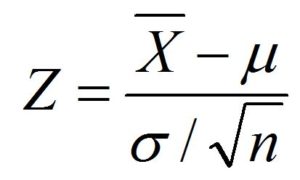
The formula used to calculate the z score is –

Here, the x could represent a raw score; however, when converting a sample average to a z-score, that raw score will be replaced with the mean of the sample, and the standard deviation of the denominator will be replaced by its average error. The formula to calculate the standard error will be:

So the formula to calculate the z score of the mean of a sample is

Examples
Below are some questions which have been solved using z scores. This will help you understand the purpose and method by which z scores can be utilized.
Question 1– A group of 50 students and there is a Math test is held. We presume that the information derived from this test’s results is generally distributed (because of the Central Limit Theorem). The test that was of 100 marks resulted in one outcome in which the mean score was 60/100; however, the variation (fluctuation in the marks of the student) was around 15. (Standard Variation).
The question is: If student A gets 70% marks. Did he perform very well? From which students did his marks are higher, and from which students did he score less? i.e., what is his score? be in relation to other scores within the range of distribution. Second What are the top 10% of students?
In the end, if student A had scored 72 marks in the Science examination, will this mean that he scored less on his maths test if the mean score of the Science test is 68, and it is the normal deviation of 6?
Answer 1: For question 1. To answer the query, it might appear that student-A’s marks are great since they are higher than the average for the class. However, we must also keep the variance of marks in mind, and we can examine his marks according to their position within the distribution. Probability distributions are a good option. Probability distributions aid in calculating an appropriate score for a specific distribution. In this case, we’ve assumed that marks for students are normalized; therefore, we apply the normal distribution standard and determine its z-score.
To determine where the score of student A compares to others in the class, compute the scores of the student as a Z score. In this case, the mean is 60, the normal deviation is 15, and an individual’s score is 70. Therefore, the z score of student A would be 0.6667.

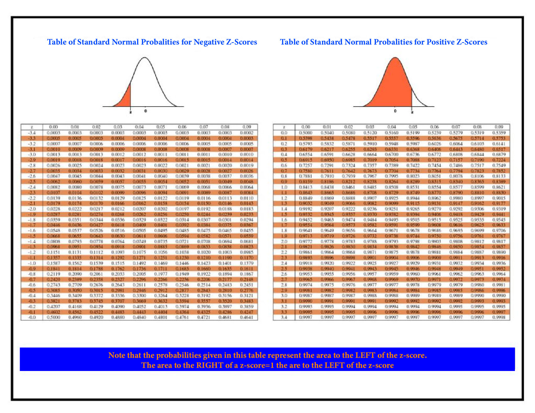
Then we can employ our Standard Normal Distribution table to determine whether a score is higher or lower than our Z score, which was 0.666. The y-axis on the table shows the first two figures of our z score, and the x-axis is the second decimal point.

We will use the table above (Right) and calculate the score. It is 0.7486, and when we multiply it 100 times, it is 74.86. This means that about 75% of our data is left side of the score, i.e., approximately 75% scored less points than students A. To find out the percentage of students who scored higher than A, we can make use of to use the Inverse Standard Normal Distribution table (or think of the z-value as being negative and apply the Table of Standard Normal Probabilities for negative Z-scores), which will give us information about the area beneath this curve, which is located on the right of our Z score. The final results are 0.667 when plotted against a standard normal distribution. Or, you can subtract 100 from 74.86 and find that 25.15 percent or around 25% of students had higher scores than student A.
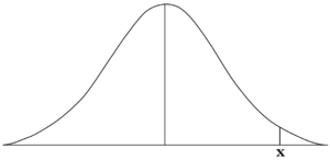
In order to answer the second question, which demands us to identify the top 10% of students, we could assume a point X from our normal distribution and determine what X’s value is the form of score z, on which the right-hand side 10 percent of the data is or falls within the curve of distribution.

We can examine the Standard Normal Distribution table and look for scores that are close to 0.9000, and then we finish getting the most close score of 0.8997, and when we look at the x – and y-axis, we can calculate that the score for z will be 1.28 (1.2 (y-axis) plus 0.08 (x-axis)).
We now have the score z average, mean and standard deviation, and it is easy to determine the score.
Z = x – m/s (formula to determine the z score when the x value is already known)
x = m + (z) (s) (formula to find x when z score is already known)
60 + (1.28) (15)
60 + (1.28 x 15)
60 + 19.2
x= 79.2
Therefore, the students with a grade of greater than 79.2 are among the top 10% of their class.
To determine the solution to the final question, we have to determine whether Student A scored higher in his Science test; we will need to calculate the Z scores of his Science marks and then examine them against the scores from the Maths Exam to find if the student actually scored better or not.
To calculate the Z score for his Science marks, we subtract the average marks from his science class from the marks of each student and divide it by the variance (standard deviation) of his score on his science test (72-68/6), which turns out to be 0.67. 0.67, which is exactly the same score that was scored on the Math test. So, student A didn’t do higher than his science test.
There are many other questions that could assist us in understanding how beneficial Z scores are to us.
Question 2- What is the percent of students who have scored marks between 567-617 in the case where the mean of this normal distribution is 517 and the average deviation of 100?
Answer 2. We first look up the z score for both marks.
z = x – m / s
Marks 1: 567-517/100 = 0.50
Marks 2 : 617-517/100 = 1.00
Then we will examine our Standard Normal Distribution table to identify the area of the curve for every score. The proportion of students scoring lower than 567 (i.e., the percentage of data that is to the left of the score of 0.50 when plotted using a standard normal distribution) is 0.6916, i.e., 69.15%. For 617 scores, it’s 84.13 percent. Thus, the percentage of students scoring between the 567-617 marks is (0.8413-0.6915) 14.98 percent.
Questions 3- What percentage of students scored higher than 130 on a Math test in which the normal distribution’s mean was 100 while the normal deviation was 15?
Answer: There are two methods of doing this: Calculating the area under the curve by using the Standard Normal Distribution table or by employing Inverse Standard Normal Distribution.
If we employ the Standard Normal Distribution table, we can calculate the percentage of students who scored lower than 130 (data below the Z score) and then divide the 100th percentile to find those who scored higher than 130.
We will apply the value of the z score in the form (130-100/15 equals 2.00); if we examine the Standard Normal Distribution, the students who scored less than 130 turn out as 97.72 percent. Thus, 2.28 percent (97.72-100) of students had scores higher than 130.
Another option is to use The Table of Normal Standard Probabilities for negative Z-scores. We will consider the value of the Z score to be negative, i.e., -2.00, to determine the value that is to the right of the Z score if it is plotted using a standard normal distribution. If we examine the Standard Normal Table Probabilities of Negative Z-scores to identify the percent of students who scored over 130, it is calculated as 2.28 percent.
Probability Distribution and Z Score
It is now clear how to calculate probabilities by using The Standard Normal Distribution. The word probability refers to an area. As we discussed earlier, all the area in a typical normal distribution is one. Thus, the probabilities we calculate will always be lower than 1.
Examples
A few questions below can assist in understanding how z scores and probability distributions work together to identify probabilities.
Questions 1. Which is the probability Z has below -1.32 on a Standard Normal Distribution.
Answer: Here, to determine the P(z = -1.32), we have to look first at our Table of Standard Normal Probabilities for Z-scores with Negatives since the score we have is positive (i.e., in the middle of the range). In addition, if we determine the probability that z is less than -1.32, we can figure out the area left of the score. If we look at the Table of Normal Standard Probabilities for Negative Z-scores, we discover that the area below the curve will 9.34%. 9.34 percent (the value listed in the table is 0.0934).
Questions 2. What is the chance that Z is greater than -1.32 on a Standard Normal Distribution?
Answer: We must determine P(z greater than -1.32), and here we also utilize the table of standard normal Probabilities for negative Z-scores; however, this time, we must find the probability of having a z score higher than -1.32. Therefore, we need to determine the right-hand side of our z score, and since our table will only provide us with the area that is left and we are able to subtract the number divided by one (Total Area under Curve) to calculate the right side which is (1-0.0934 = 0.9066) 90.66 percent. So the likelihood of having a score higher than -1.32 is 90.66 percent.
Questions 3. What is the likelihood of z falling somewhere between -1.28 and 0.72 in a normal distribution?
Answer: The answer to this question is easy. Find the area left of -0.21 and 0.85 and subtract them to get the portion between. The area left of -1.28 (using the Table of Standard Normal Probabilities for Negative Z-scores) is 0.1003, i.e., 10.03 percent, while the portion that lies to the left is 0.72 (using the Standard Normal Probabilities Table for Positive Z-scores) is 0.7643, i.e., 76.43%. Thus, the gap between them is, i.e., 66.39%.
Question 4. Another relevant question is the likelihood of an adult who is randomly selected American female being larger than 170.5 cm when the mean of the mean is 162.2 cm and the mean deviation of 6.8 centimeters. 6.8 centimeters.
Answer: Here, we need to determine the Z score, which is 170.5 cm. Then we need to determine the area that is to the right of the score. Therefore, the z score is 1.22. The left-hand side will be 88.88 percent, so it will also comprise 100-88.88, i.e., 11.12%. The probability of locating this female is 11.12 percent. (Here, we also can infer that this score of 1.22 implies 170.5. 170.5 represents 1.22 standard deviations above the average of 162.2 since the z score shows the standard deviations of an individual’s score is in excess of and below the average.)
Z Test
Z Test is a hypothesis test founded on Z-statistic, a normal distribution that follows the standard with the null hypothesis. The Z-value discussed above is a “test statistic for Z-tests that measures the difference between an observed statistic and its hypothesized population parameter in units of the standard deviation.”
Z Tests are utilized in many scenarios, like the one-sample z-test, which tests an average of a distributed population in which a standard deviation is established. It can also be used in Regression to determine whether the variables that predict (independent) variables are significant for the dependent variable or not. Z Test is also used to perform an approximate normalization for tests of Poisson rates and test of proportions. Therefore, Z-Test is utilized to test of hypotheses in scenarios.
- Testing refers to situations where there is a normal population, the sampling size is high, and the variance is well-known.
- Testing Differential means when the population is normal, the sample size is high, and the variance is well-known.
- Test of Proportions or Difference between proportions (Used for quantitative data)
- Test the difference between proportions
Z Test is used in hypothesis testing. In the following blog, the z values from Z tests will be utilized to conduct hypothesis testing, where probabilities are calculated to reject or accept the hypothesis.
The question above (Question 4, under the heading ‘Probability Distribution ‘ and Z Score’) used the Z values to determine probabilities. More information about Hypothesis testing can be found in the coming blog for this topic, but to give you a concept, the same question as the one above in Hypothesis Testing will appear similar to this:
A typical height for one American woman is 162.2 cm, with a typical deviation of 6.8 centimeters. A recent study of American women, with an average of 200 women, discovered that the median height is 170.5 centimeters. The average height of American women been increasing?
We will apply the same formula and employ a Z-test; however, the method of drawing inferences will differ and will make use of terms like Null Hypothesis or Alternative Hypothesis P-value, and so on. (More about this in Hypothesis Tests).
Other Probability Distributions
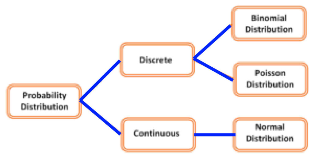
Other than the most commonly utilized probability distribution, the Normal Distribution (aka Gaussian Distribution), There are a variety of Probability Distributions.

Different kinds of probability distributions are, for instance
Binomial There are only two possibilities with the likelihood of success being identical across every trial, with each being distinct. Example: Distribution resulting from throwing the coin.
Poisson is an unidirectional distribution. It is the term used to describe the number of events happening within a time-span or area of potential. Example: How many people go to a site of monuments that opens from 9:00 am until 5 pm?
Other distributions may include Hypergeometric, which works very similar to Binomial; however, it’s not precisely 50-50% for an outcome, but it is fluctuating across. One example could be: Five cards, there are how many spades in the deck? With each choice, the probability changes. There are numerous kinds of distributions to investigate further, including Log Normal Chi-squared, Gamma Beta Weibull, and Exponential. Negative Binomial and so on.
The blog article discussed some inferences that were drawn; however, the aspects of the data weren’t explained. The theories discussed in this blog post will be applied in the coming blogs.
