ARIMA represents Auto-Regressive Integrated Moving Average. It is a high-level method that is employed for forecasting. Similar to the ETS, ARIMA also requires the data to be stationary, and If the data is not stationary, it will be transformed into stationary. ARIMA is described with three orders of parameters referred to as p, d, and q which means that AR is represented by p. I represent d, and MA can be represented with the q. The ARIMA procedure is referred to as the Box-Jenkins method (the procedure of making the model into an ARIMA model is known as this). ARIMA can be described as a stochastic method, i.e., the data must remain stationary to ensure that its properties are not affected by a change in time.
ARIMA family
There are many types of techniques that belong to the ARIMA family and were briefly reviewed below.
Auto-Regressive (AR)
In this way, the future value is based on the value that was previously used. This is mathematically known as
Yt = c + a1 Y t-1 + et , -1 1<1
In this case, the auto-regressive parameter indicates how many lags are used (the number of values from the past to be considered) in the process of making use of the models.
The mathematical equation that governs an AR procedure is
Yt = c + a1 Yt-1 + a2 Yt-2 + a3 Yt-3 . . . a p Y t-p + e t
Moving Average (MA)
The values forecasted here depend on the error numbers from the past i.e.
Yt = c + et – b1e t-1 , -1 1<1
This parameter is a variable that determines the number of terms that will be used in the calculation, i.e., the number of past errors to be considered in making the forecasted value, which creates an equation of Moving Average Process look like: Moving Average Process looks like:
Yt = c + et – b2 et-1 + b2 et-2 + b3 et-3 . . . bq et-q
Auto-Regressive Moving Average (ARMA)
This method is only utilized when the dataset is static. This technique is a mixture of AR as well as MA and, when both methods are combined it is possible to be left with ARMA. Two parameters are utilized to define how many lags, and q indicates the number of terms.
Auto-Regressive Integrated Moving Average (ARIMA)
ARIMA can be described as an expansion of ARMA in that ARMA is only able to be used with static data, whereas the ARIMA model is able to be used on non-stationary data. This is achieved through the use of difference, which is employed to make the data stable in ARIMA. In this article, we introduce a second parameter, called d, which controls the time it is necessary to alter the data to ensure it is stationary. It is the ARIMA model that functions as a non-seasonal model that makes use of all three of the components: Autoregressive (p) and Differencing (d), as well as moving average (q) to construct this model that is not seasonal. ARIMA model.
When you combine all three, the mathematical equation that explains the ARIMA process turns out to be:
Yt = d + a1 Yt-1 + a2 Yt-2 + a3 Yt-3 . . . ap Yt-p + et – b1 et-1 + b2 et-2 + b3 et-3 . . . bq et-q
It is essential to remember in the use of ARIMA that when any parameter (p,d,q) is zero, the method applied changes as we remove the component from the model. For instance, if in our ARIMA model, the value for p is 2 and d and Q is zero, then the algorithm employed is just Auto Regressive because the differencing and moving average component is not present.
Determining Stationarity of the Data
As stated above, the main requirement to be eligible for ARMA requires that data must be stationary. What is meant by stationary is the fact that data must not exhibit any trend, i.e., the data has a constant autocovariance, variance, and mean across the period. The data has to be stationary to support ARMA since previous values influence the nature of the two processes: AR and MA. So, we require data with properties that are consistent throughout time. Thus, the requirement is that the data be stationary.
Graph
The typical graph for static data appears to look something like this:

In this case, the data fluctuates using the same standard deviation and constant mean, and there isn’t a trend.
It is important to note that any irregularity in the standard deviation, regardless of whether trends are absent, is not considered to be data being stationary since the fluctuation between different times of data points creates irregularities, and this variation must be consistent.

So, the simplest method of determining if it is stationary is just by taking a look at the graph.
Augmented Dickey-Fuller
Another option is to perform the Augmented Dickey-Fuller (ADF) test, which is a statistical significance test in which the null hypothesis states that the data isn’t stationary. The alternative hypothesis is the information is stable. This test is also referred to as the Unit Root test. Other methods include Ljung Test etc.
Auto Correlation Function (ACF) and Partial Correlation Function (PACF)
Another method to determine whether it is not stationary is discovering the trend component with techniques like Auto-Correlation Function (ACF) and Partial Auto-Correlation Function (PACF).
Auto Correlation Function (ACF)
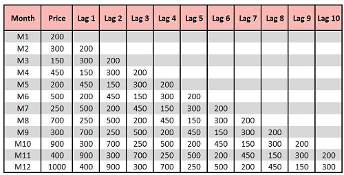
As was mentioned previously in previous blog posts, as mentioned in the earlier blog in the previous blog, the trend is simply outlined through the line of regression. If, for instance, you have a price variable and 20-time intervals, we must determine that the price increases by a certain amount in that time period (if the shift from 1 time period to) What amount of increase can be seen on the cost? This is how we perform Regression, i.e., with one unit of x, the change in the value of y. Thus the trend is the Beta component of the linear equation. Therefore, we calculate linear trends in which price is the present value for the price variable is a subset of the earlier value of the variable ‘price’. In this case, we are able to see an idea of autocorrelation forming. When we examine the following dataset, which includes the time intervals M1, M2, and M3 …, in accordance with autocorrelation, we can conclude that M2 is dependent on M1, while M3 is a result of M1 or M2 and the list goes on. In this way, we are able to have the idea of lag, where for Lag 1, we take into account the initial value, for lag 2previous to the value before and lag 3 prior to the previous value, and so on.

If we determine the correlation between price and the Lags (for instance, correlation(Price, Lag 1)), (Price, Lag 2) . . . . . (Price Lag 59, Price)) The ideal output should show an increase in frequency. Suppose the correlations are at their highest at specific intervals (for instance, a glance at the end of every 12 (Price, Lag 59) months which indicates that the correlation is similar throughout December). In that case, this suggests the presence of seasonality. This relationship between variables and the lags is known as auto-correlation. ACF defines the degree of connection between the various data points within the dataset. It is possible to draw an ACF and make correlograms, which help to determine the order of difference (d) and the direction for the move means (q).
Partial Auto-Correlation Function (PACF)
This technique reveals the relationship between variables and their delays that are not understood (affected) by prior lags. In our case, correlation means that if the price and Lag 1 is linked, then Lag 1 and 2 are also connected. So, Lag 3 impacts Lag 2, Lag 2 and Lag 1, and Lag 1 affect sales, and that’s just the beginning. To understand the true effect on sales of Lag 1 for sales it is necessary to eliminate the effects from Lag 2 upon Lag 1. Thus, if we eliminate the prior amount (Lag 2,) and determine the correlation, this method is known as Partial Auto-Correlation. This method is utilized to determine the impact of the particular time frame. What effect will we see if we do not have the historical data available and focus on a specific time frame? Similar to ACF, we can also plot PACF, which can assist in determining the sequence of the auto-regressive parameters (p).
Methods for making data Stationary
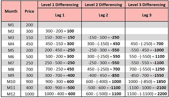
There are many ways of making data stationary; the most popular is via Log transformations that can help stabilize an ongoing trend. Another effective method is to use Detrending, which takes the differences in the series and aids in eliminating the tendency from data. We must be aware of how often we have to carry out “differencing” to ensure that the data is stationary. This gives us the value of the parameter d (I in ARIMA). ARIMA). So, if d equals zero, we don’t have to perform differencing since the data is static, and we are able to proceed using ARMA only. Below, we apply 3 levels of differencing in which level 1, we determine the difference by subtracting the current period’s value from the previous period’s value. In level 2, we add an additional lag in the series, and so on.

Overview of the Steps
A typical method of making an ARIMA model using the Box Jenkins Methodology comprises
- A visualization of the data to determine whether any seasonality, trend, or cyclicity is evident or not.
- Separate the data into what is the Trend, Seasonality, Cyclicity, and Irregularity component (explored earlier in this blog). Prior post).
- Examine stationarity by employing methods like testing stationarity using methods such as the Augmented Dickey-Fuller (ADF) Test or making use of ACF or PACF plots to determine the exact order of difference needed.
- If there is no stationarity, make use of transformations.
- If the stationarity cannot be achieved, then you must determine the order of difference by using ACF or PACF plots and execute differentiating to make the data stable.
- Make use of ACF or PACF plots to determine the sequence of AR and MA.
- Fit ARIMA Model
- Evaluate the model
In the application, the software discovers the parameters p,d, and q while determining if that data has a stationary value or not, and making it so can be accomplished in software using simple one-line codes. It is important to remember the key distinction between smoothing and ARIMA in that both require that data stay stationary. Techniques for smoothing like single exponential smoothing use only one past value and one value for error from the past; similarly, double exponential requires two of these values. However, in ARIMA, we aren’t sure about the number of past values to be considered, and in this case, the past value and the past error value could differ, so we can use two past values when considering three errors.
ARIMA is an effective forecasting tool; however, it is important to note that when using this method, it is essential to be able to access a substantial quantity of information. It also is more effective on long, stable data series. The method is the most advanced technique of forecasting described in the past and should be utilized for accurate forecasting.
