K Nearest Neighbour, often referred to by the name KNN, is an example-based learning algorithm. Unlike linear or logistic regression, which uses mathematical equations employed to predict the results that KNN can predict, it is based on instances and doesn’t employ any mathematical equation. Because there isn’t any mathematical formula, it doesn’t have to rely on any assumption like the normal distribution of data, which is why it’s a non-parametric method to predict. It’s a supervised, non-linear approach to solving classification and regression issues.
Idea Behind KNN
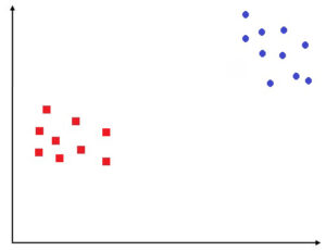
Let’s look at KNN through an example. Let’s assume we have a data set that has y variables—two classes, squares, and rounds.
There is a second unknown area (black triangular) and we need to know what class it is in. Suppose the same data is presented to a child, and it is not the computation of a prior by Naive Bayes or a hyperplane, as performed through logistic regression, or computing information gain, as performed by decision trees or decision trees. In that case, the child will examine the points near this unknown spot and determine the point belongs to that particular class. This is what KNN does when it classifies the data points based on its proximity to examples of training.
Voronoi cell
We have a set of data that is similar to the one below, where the data points belonging to different classes are located in greater proximity to what was seen earlier.
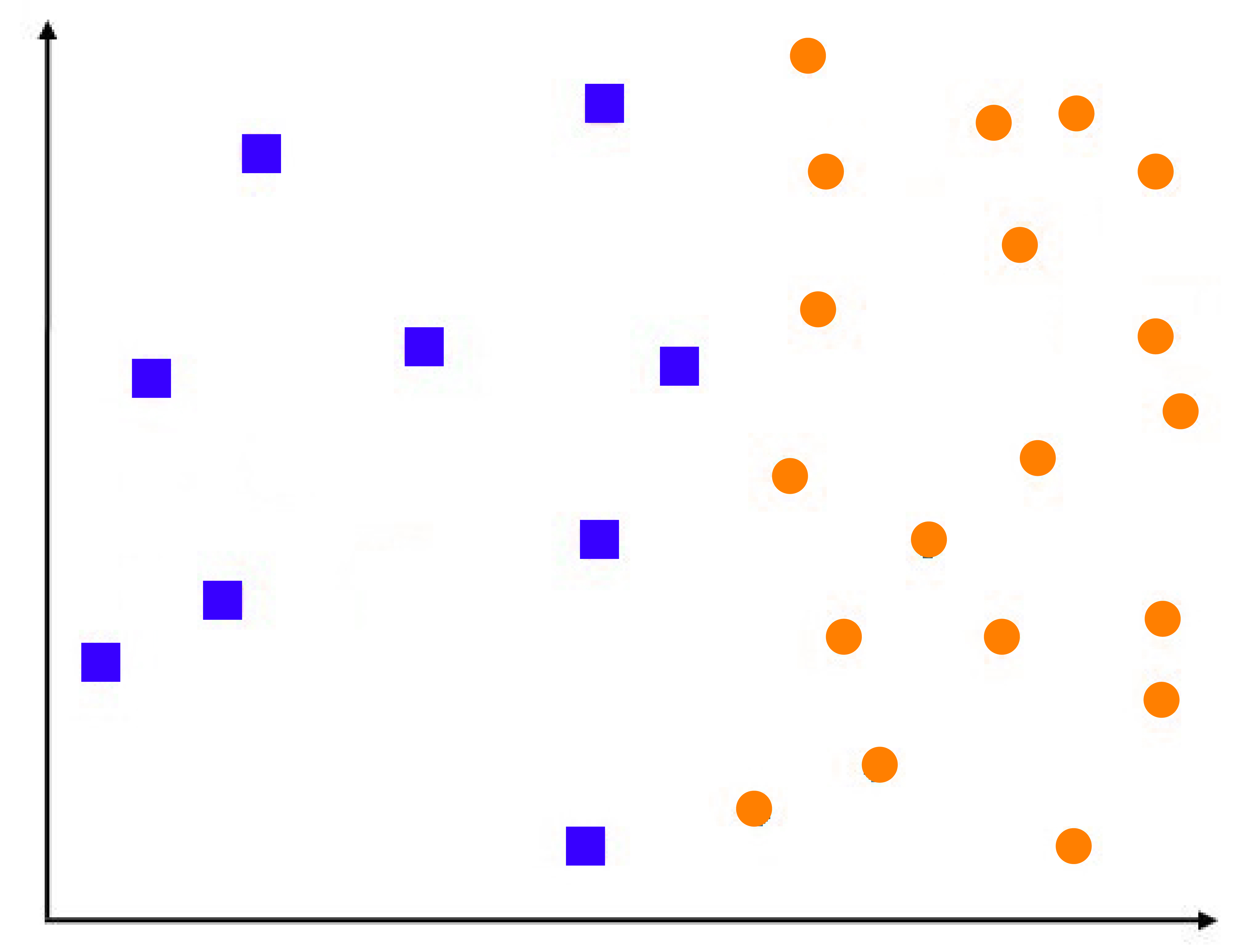
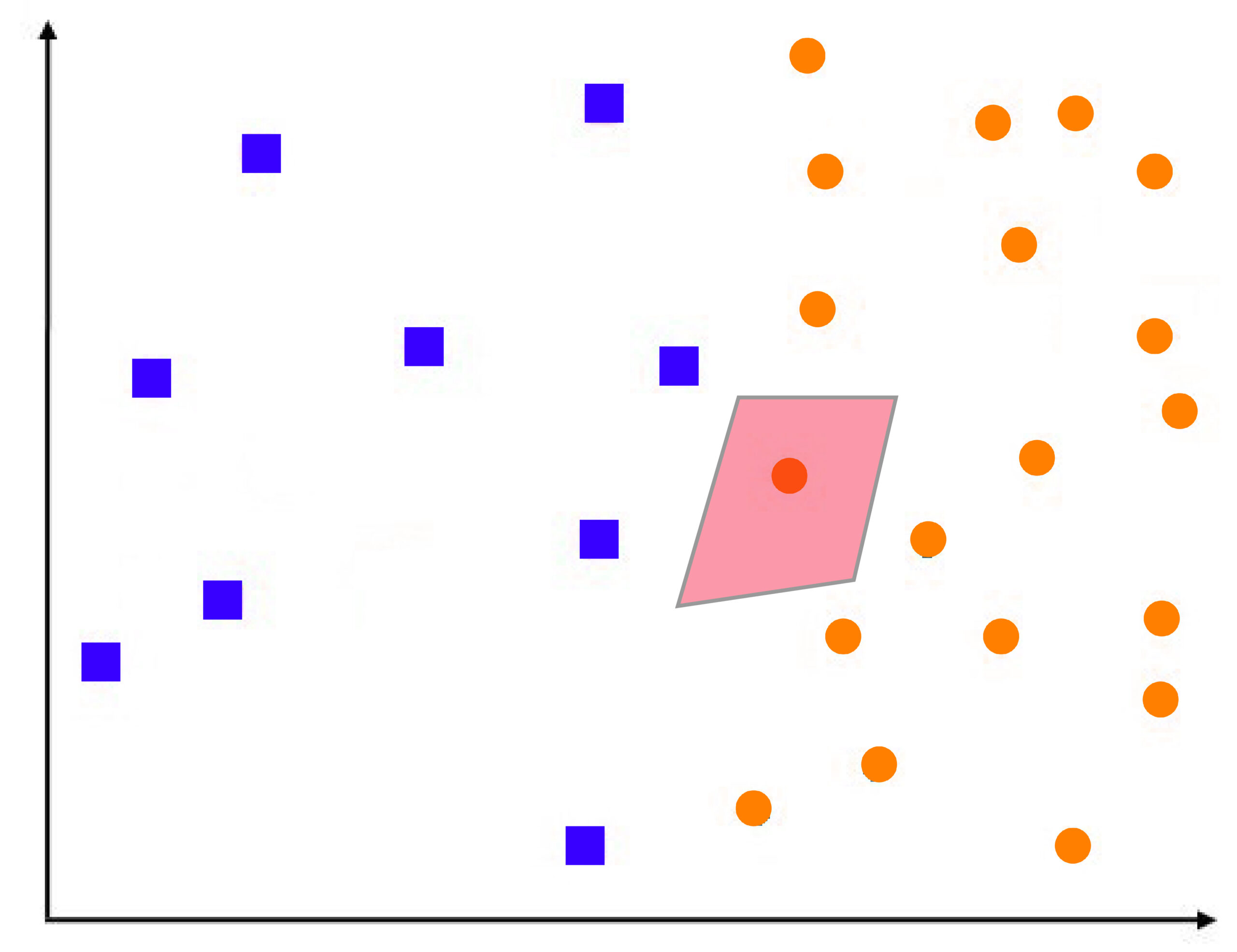
Suppose we set k=1 in our algorithm for k’s closest neighbour after every new data item. In that case, the closest training examples are found, and its class is considered a good predictor. To comprehend this better, it is necessary to understand the meaning behind Voronoi cells. The following diagram shows the way a region around it surrounds a blue data point. It is designated blue. Therefore, any point in the area or neighborhood will be classified as blue. So, an entire cell is a colored blue because of one data point. The blue area is the Voronoi cell.
The role of importance of K
In the nearest neighbor of K, the data points have a Voronoi cell that is known as Voronoi Tesselation. Now, we can develop a decision boundary passed through the cell in a way that distinguishes a particular class of data points and the other. However, K’s nearest neighbor, even though it is a very basic algorithm, has decision boundaries that are more complicated than the one that Naive Bayes, as well as Logistic Regression, have come up with and is as good as decision trees. This is what we have to address and will discuss further on this site.
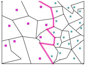
To comprehend why we employ the k=n algorithm and not stick with k=1 to predict in the first place, we must look at some of the shortcomings of the KNN model, which is that it is extremely sensitive to noise and outliers because it could result in changing the boundary of the decision quite dramatically. If, for instance, there is a blue data point to the extreme left that is due to noise or an outlier, then the boundary of the decision will change dramatically, and the entire region around the information point is labeled as blue, whereas it is clearly located in a region of the red points.
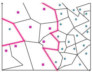
Additionally, in contrast to Naive Bayes, this model doesn’t consider the importance of a particular class and does not have any analogy to ‘the previous and ‘prior’ to assess the amount of time a class is when compared to another. This means that it does not provide any confidence value. But, if instances of data belonging to a certain class have a large majority, they will impact the majority of votes. To combat this, the number of k must be altered so that by increasing the amount of k, we can add greater security to the model.
So, let’s try to understand how the value of k affects the whole process of KNN because k=1 will make the decision boundary extremely sensitive to noise and could make the model extremely complex and insecure. Any slight change in training data will drastically alter the boundary of the decision.
It is possible to increase the value of k, as an example, by 20. What we mean with 20 is that for an unidentified data point, it will consider more than one closest neighbour, i.e., it is now looking at 20 neighbors to establish its classification. In this case, the predominant class is taken into consideration for prediction, while the means to determine a class’s dominance will be discussed in depth.
In the past, increasing k makes the model simpler; however, if we choose the appropriate amount of k, say that k= no. of samples, it will be able to sort on the basis of the type of class that is frequently used when transforming the model into a prior classifier. So, a huge number of samples will cause the model to underfit. To determine the correct value for k, we employ grid search, cross-validation, and resampling.
If we look at these figures, we will see that with a lower value for K, the model is an example of overfitting and can be very difficult to be able to generalize. However, increasing K’s value smooths the boundary of decision-making and improves the stability of the model.
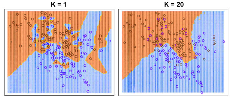
The decision boundary is very less complex for a higher value of k
Working of KNN for a Classification Problem v/s Regression Problem
Classification Problem
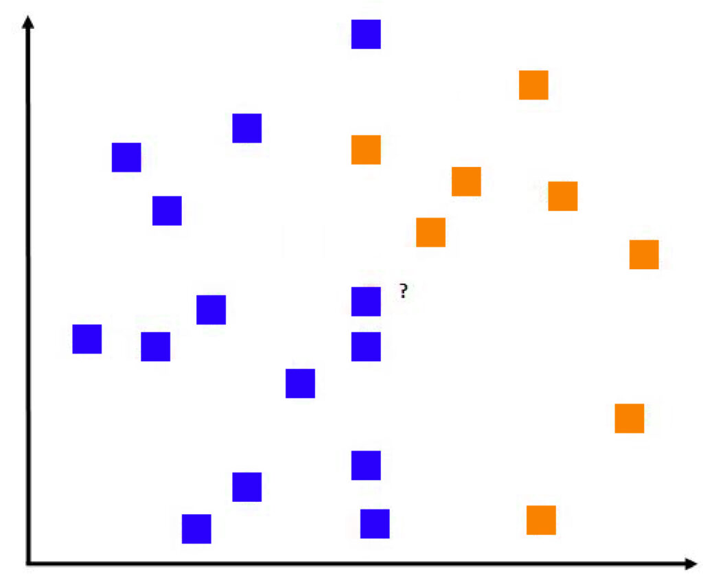
Below is the information with two classes, Red and Green, and we must identify the class in Yellow Box. Yellow Box.
In a classification issue in a classification problem, we select the element that we wish to classify and begin computing the distance between the unidentified data point to each data point in the dataset used for training. We then select k of data points closest to the data point and then, based on the most frequently used class, give the data point with the unidentified data point. Therefore, we apply a majority vote method to determine the classification of the information point.

The number of Data Points considered is completely based on the value of k.
In the above diagram, when the value of k was 1, the data point closest to the square was yellow red; therefore, it was labeled as a red data point. When we increased the value of k by 3, it could get the three closest data points to it. Of these, two were red, and one was green. If 7 was the value of k, we had 4 green and red, while when k=13, we got 9 red and four green points.
Regression Problem
If the labels to be predicted are continuous, and continuous, then the KNN Regression method is utilized.
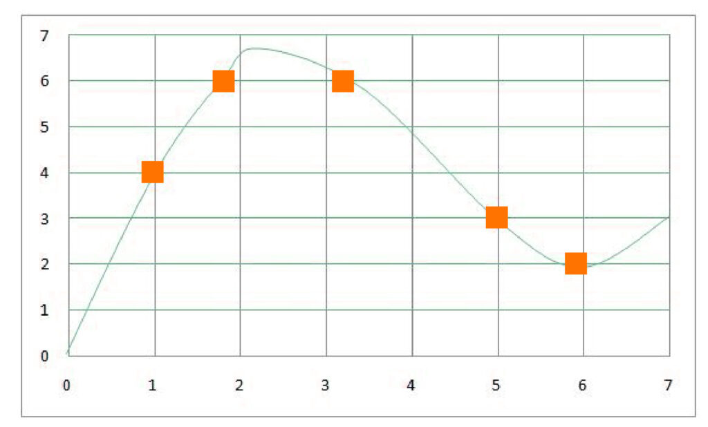
In this case, we also use the unknown point to calculate distances to all data points and then find those closest to the data point. Instead of voting with a majority to decide, we use the mean of the Y variable, which the closest data point represents, so that we compute the mean of the label of the close neighbors. This mean is used to determine the prediction. We have here the 1-dimensional representation of the regression problem. We need to determine the real function that is not known to us. The next step is to try to predict this function based on our data.
On the x-axis, you have the numbers we are trying to predict, and on the Y-axis, we can see the different numbers of the Y variable. If we have a number of inputs, if we need to predict the Y, then we will look at the x-axis to find the point closest to it (we don’t examine the y-axis because it represents the Y variable and isn’t the sole basis for prediction, we’re forecasting Y on the basis of the x). The closest spot to 4 is 3.2, which means that if we’re using k=1 as a parameter in the algorithm, this point is considered as a Y-related point, and the associated Y label will be used to determine the value. So, for a value of 4, the Y value will be calculated as 6.
However, if we employ the k=2 algorithm, then we take the two values closest to the x variable (which comprise 3.2 and 5 and make an average of their respective Y variable, which is found to be 4.5 ((6 + 3) + 2 = 4.5). Therefore, for an equation of x=4, if two ks and Y=2, the value would be 4.5. It is possible to do similar calculations with different values of k. We will choose the value of k which provides us with the prediction that is closest to the actual function.

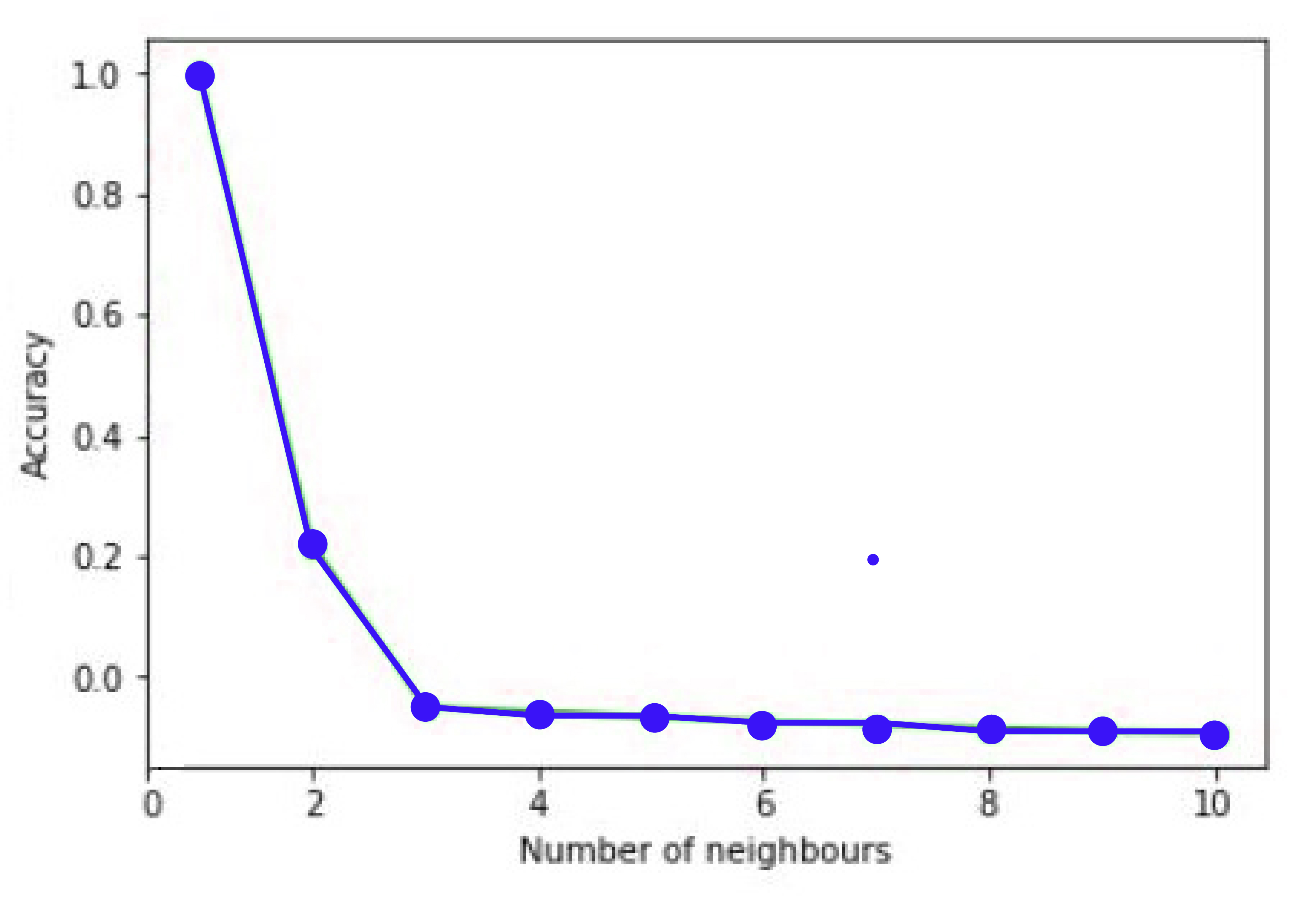
Predicted values based on different values of k
Accuracy v/s Number of Neighbours
It is evident that k=2 yields the best results. Therefore, we can observe that determining the correct value for k is extremely important because, with a low value, the model gets more complicated. In contrast, the very high value of k, such as k=total number of samples, then it will result in the average of the variables Y.
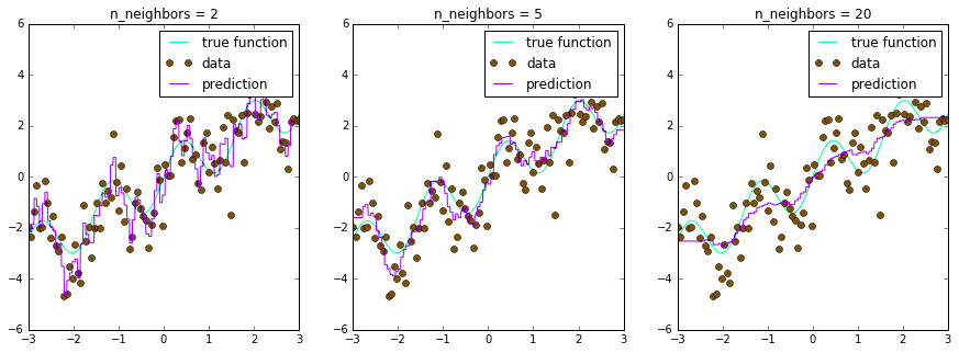
True function v/s Predicted function for different values of k
As previously mentioned, We can utilize grid search to determine the parameters of k, and then determine the one with the greatest accuracy.
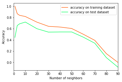
Accuracy on Training Dataset v/s Accuracy on Test Dataset for different values of k
Methods of Improvement
So far, we have looked at the significance of KNN as a hyper-parameter that can be adjusted to produce more efficient results. But, there are plenty of possibilities in dealing with KNN since there are numerous parameters and ways to improve that could be employed to give us more efficient results. One of these is the following:
- Using different Distance Metrics
- Alternatives to Majority Voting
- Techniques to Approximate Nearest Neighbour
- Resolving Ties
- Rescaling Data
- Missing Value and Outlier Treatment
- Dimensionality Reduction
Distance Metrics
Based on the type of feature KNN is working with, altering the method used to calculate the distance could greatly improve the accuracy of the results generated by KNN. There are a variety of distance metrics apart from the standard Euclidean Distance used so far like, Hamming Distance, Minkowski distance, etc. The blog KNN Distance Metrics for more details.
Alternatives to Majority Voting
In the past, the method for the majority vote was used, but this option can be accompanied by its own disadvantages. Hence, alternative methods to majority voting are available that can aid in improving the results that are generated using the method. For more details, refer to KNNAlternatives to Majority Voting.
Techniques to Approximate Nearest Neighbour
One of the main negatives of KNN is that it’s extremely slow during the testing phase, making it difficult to use. The primary reason is that it uses all the data points in the process of approximating neighbors, which makes the entire procedure extremely slow. Various methods like K-D tree, LHS, and Inverted List could be employed to make the entire process more efficient without losing any precision and reliability. They are being the study within KNN- Methods to approximate nearest neighbours.
Resolving Ties
If there is a similar number of votes from various classes, it isn’t easy to choose one class to predict the data point that is not known. If the classes are binary, the equal value for k must be avoided because the even number of values could cause the formation of ties. Thus, the values of k ought to be unusual (1,3,5,7,9 . . .). But this method will not be used for multiple class problems, and in such situations, we must be careful to prevent the value of k from being the multiplication of the class number. If there is a tie, we can change the value for k to one or choose the class randomly. A more reliable alternative method would involve prior, in which the class with the highest frequency overall is taken into consideration for prediction.
Rescaling Data
When data is used in an analysis based on distance has to be scaled up. For instance, there are two variables: the height of the individual in meters and the weight of the one in pounds. Since the weight’s absolute value will be higher than the distance metric, it will be distorted. Thus, various Rescaling Methods can be employed to rescale features prior to using them in KNN. To learn more about the various scaling techniques, check out Feature Scaling.
Missing Value and Outlier Treatment
Extreme values and missing values are extremely harmful to the KNN. The models that utilize distance metrics are affected by outliers, and outlier treatment has to be carried out on the data before using it in the KNN model. Similar to missing value treatment needs to be applied to the data to ensure that KNN is able to be properly executed. See the Missing Value Treatment as well as Outlier Treatment for more details.
Dimensionality Reduction
If there are lots of unimportant factors (causing multicollinearity) and unlike decision trees that ignore these variables and aren’t negatively affected, KNN is negatively affected because it assigns equal weight to every feature. Therefore, if the data are in extremely high resolution, KNN isn’t working correctly. Consequently, feature reduction methods should be used to improve the accuracy of the distance metric, making it more useful and the model more reliable.
Pros and Cons
Like other algorithms similar to the KNN, KNN is not without its advantages as well as drawbacks.
Pros
It requires no assumption, i.e., It’s a non-parametric approach, meaning it doesn’t require any assumptions, i.e., we don’t have to. It is suitable for regression and for the classification of multiclass binary issues. The time spent by KNN in the training process is considerably less compared to other models, and it is more efficient in generating these complicated results. Additionally, it is easy to grasp and simple to apply.
Cons
It’s not working correctly in the event of data that is not complete, or outliers are excessive features that are not needed or aren’t scaled. Another issue for KNN is that, unlike ANN, which is slow during learning and quick in training, KNN is relatively fast in the initial phase of training it is compared to the testing phase, where it is very slow. This is because, unlike other models, where a function is learned and later applied to the test collection, KNN remembers every instance of training. These instances can be described in terms of the number. In the testing phase, the test samples are compared to the number. Therefore, it renders the process extremely computationally demanding.
Additionally, as the amount of training data increases, the training process gets slow. If you are using majority voting results, the outcomes could be distorted because the classes frequently found in the data will be dominant in the majority vote. This is why other methods like weighted voting might be needed.
K Nearest Neighbour is an extremely simple and effective technique that gives us numerous possibilities to expand our model. It is a great tool for Classification and Regression issues. It is prone to being prone to overfitting and slow, but there are a variety of ways to overcome it. The hyperparameters mentioned in this blog should be considered to find the KNN model that suits your data and gives excellent results.
