A Decision Tree can be described as “a decision support tool that uses a tree-like graph or model of decisions and their possible consequences”. In this blog, we will look at the algorithms that are based on decision trees employed for prediction or classification. Decision Trees are a complex analysis since it can be difficult to determine when to use them. They are used when data is of poor quality. Tests like Hosmer Lemish tests may be used to determine whether the data is appropriate to be used for logistic regression or not. When data is complex, or the issue is complex and hard to communicate to clients, decision trees are a good option to provide an element of control for the classification process. In contrast, logistic regression is an opaque box in which we introduce the data and output the result. Additionally, decision trees are not affected by outliers or insufficient values or the need to transform data because they attempt to use all thresholds that are possible and every possible feature and thus are extremely robust in this regard.
Regression Trees v/s Classification Trees
Decision Trees are of two kinds: Regression Trees and Classification Trees. Regression Trees are employed when the dependent variable has a constant variable, and we must predict its value. Classification Trees can be utilized as a substitute for logistic regression. In this case, Classification Trees such as Logistic Regression are able to be utilized to determine if a mix of x variables has the Y=1 value or not. Suppose a dependent variable is binary or a variable comprised of just two categories, a method known as CART or CHAID is utilized in the case of a dependent variable that contains more than two categories. In that case, the classification tree is based on an approach known as C4.5.
A great example of how to comprehend classification trees could be an example of a data set where one of the variables is whether or not a pupil in grade 9 is chosen to attend a basketball training camp, or not. As for the independent variable, we can determine the students’ height, weight, and scores. The classification trees are now required to determine on the basis of these three variables which students will be picked to participate in the basketball training camp or not. The Classification Trees first classify students based on criteria that serve as the primary factor in determining whether students will be chosen. The homogeneity of the data is taken into consideration. For example, if the decision tree shows that 95% of students with a height of more than 1.73 meters are chosen for the camp, the data is 100% pure. Different measurements (such as Chi-square, Gini index, entropy as well as entropy, Gini index, etc.) are considered to make the decision as pure as it is. This binary split of data is the basis of the process of creating the classification tree.
However, Regression Trees can use techniques like CART when the dependent and independent variables share a linear relationship and C4.5 in the event the relationship isn’t linear. CART (does binary partitioning recursively) is employed to keep the splits pure by making each cycle of the algorithm used to create a regression tree (algorithm, for instance, being Reduced in Variance) is used for each of the independent variables, find the most effective cut off point called’s so that, if we split the data into two, the average Square Error of the samples below’s as well as the square error for the samples that are above ‘s’ will be minimized. After this has been done for all the independent variables, the selected variables provided the most (lowest) mean Square Error. To determine the first split, every independent variable is divided across multiple points, the error is analyzed (the variation between the predicted value and the actual values), and then the split point with the most error is selected to divide the data. This process repeats until the next step will yield a small gain on the MSE.
One should be aware of the fact that classification trees are typically known as Decision Trees exclusively because the Decision Trees are typically used for classification, and that is why this post is going to predominantly examine classification trees while occasionally touching upon the subject of regression Trees.
Advantages of Decision Trees
Decision Trees offer high precision and require minimal preprocessing of data, such as outlier cap and missing value, variables transformation, etc. Additionally, they can be used in cases where both the independent and dependent variables aren’t linear, i.e., it can capture non-linear relations. They require less information than an analysis of regression requires. They are simple to understand and are extremely curious. Tree-based models can be easy to visualize using clear-cut demarking, making it easy for people without knowledge of statistics to grasp the procedure easily. Decision Tees are also employed for data cleansing, data exploration, and the creation of variables and selection. Decision Trees are able to use categorical and continuous variables.
Greedy Algorithm
It is believed that the Decision Tree follows a Greedy algorithm. If, for instance, the algorithm chosen is chi-square, then within the greedy algorithm, at every stop, it performs a chi-square and determines whether the independent variable can be connected to the dependent variable or not. This is why it considers all variables and picks the one with the highest purity and ‘clean’ split. This is why it determines the most effective solution for each stage, then repeats the process to determine the most optimal solution for the particular stage.
Important Terms
- Decisive Node Each node that splits is referred to as the decimal node.
- Root node It is considered to be the most important decision node and is the whole sample, which is then divided.
- Leaf Node Sometimes called the Terminal Node; it is a single node that doesn’t break further.
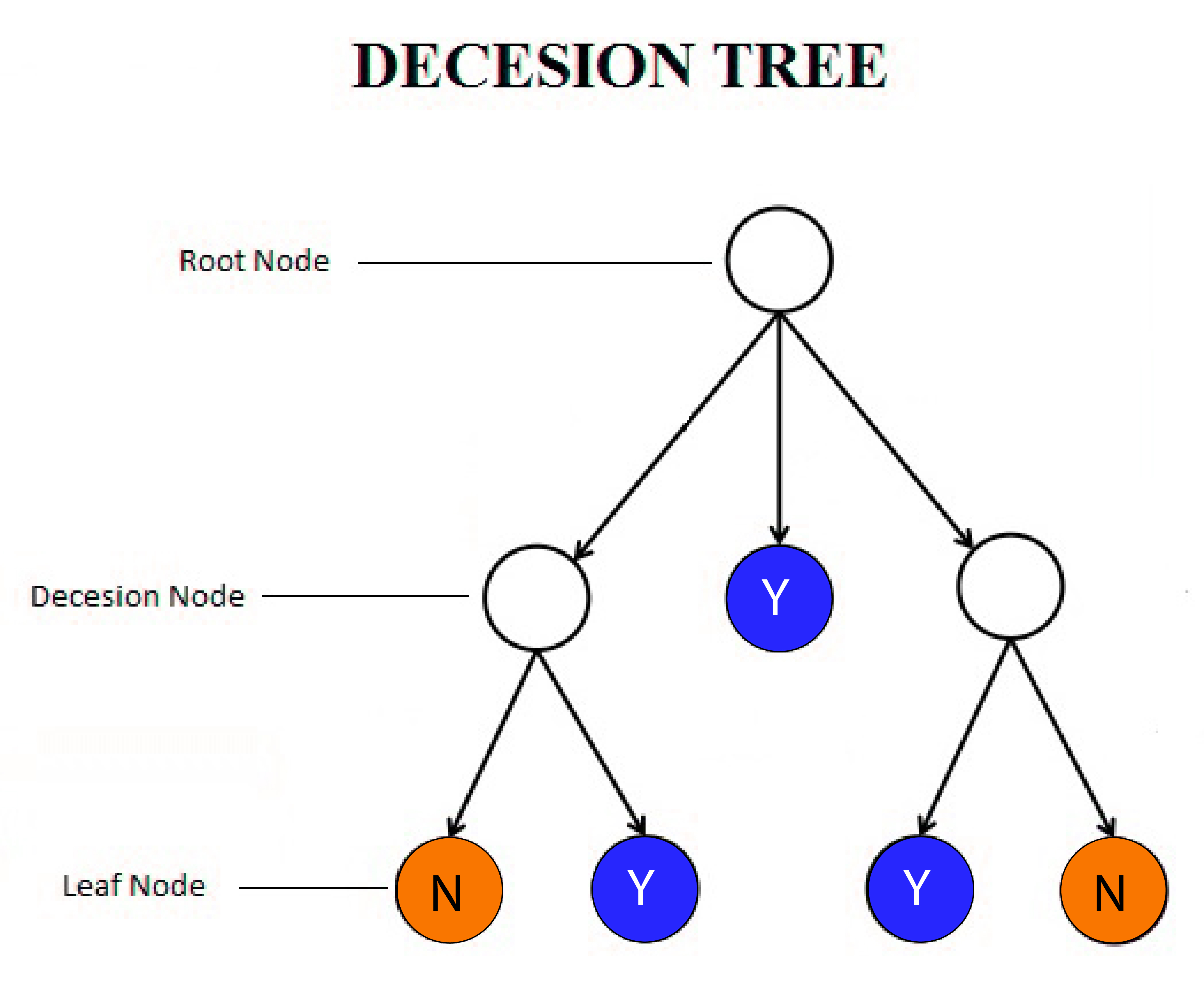
- Parting: The splitting of an element is referred to by the term “splitting.
- Pruning is exactly the same as splitting. In this case, we eliminate sub-nodes of the decision node.
Methods for creating Trees of Decision Trees
As previously mentioned, There are various methods by that decision trees can be built. Each of these techniques employs specific algorithms as decision criteria to improve the homogeneity of sub-nodes. It is a subject we will discuss more within this post.
There are numerous well-known methods like
ID3: ID3: Iterative Dichotomider 3 is the principal algorithm used to construct decision trees. It is based on the top-down method (splitting). It employs Entropy (Shannon Entropy) to create the classification trees because ID3 utilizes a top-down approach that is prone to the issue of overfitting.
C4.5 This is the successor to ID3. It is employed for the classification of dependent variables that are classified into more than two categories. It is utilized to build regression trees in cases where the relationship between the dependent (Y) and independent variables (X) does not appear to be linear. It is a significant improvement over ID3 since it was able to manage categorical as well as continuous dependent as well as independent variables. It can also overcome the problem of overfitting (discussed in this blog) using the bottom-up method (pruning ).
C5.0 Certain improvements were implemented over C4.5 This included improved speed and memory usage, and most importantly, the addition of the boosting algorithm
Cart: One of the most popular methods, it is a non-parametric algorithm for learning a decision tree in its entirety. Its full name is Classification and Regression Trees. It’s like C4.5; however, it uses the Gini Impurity algorithm for classification to ensure that each node is as pure as possible.
CHAID Chi-Square’s automatic interaction detector precedes ID3 by six years. It is a good choice for classification and regression trees. It is a non-parametric method since it employs chi-square as the measurement to create the classification trees.
Other Algorithms employed in decision trees are MARS CRUISE, QUEST, CRUISE, etc.
Algorithms of Decision Trees
The many decision tree algorithms discussed above employ various methods to divide the nodes. Various algorithms are used to decide this ‘decision criteria.’ ‘
The most commonly used Criteria/Metrics used to be used in Classification Trees are:
- Gini Index
- Entropy
- Chi-Square (for Classification Trees)
- Reduction In Variance (for Regression Trees)
- ANOVA.
To better understand how these strategies are implemented, we will look at the data that was described earlier. As the dependent variable, we can determine whether or not the student’s selected to coach basketball at school. In order to determine the independent variables, we will use two categorical and one constant variable. The categorical variables will be the Academic grade (A or B, and C or D) and the class of students (9th and 10th classes), while the continuous variable is Height.
Metrics for Classification Trees
Gini Index
It is employed in CART and does Binary splits.
The formula to calculate Gini Index is
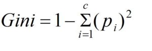
In this case, we add the probability of ‘pi’ in an item that has the label “i.” It reaches its minimal (zero) in the event that all the cases in the node fit into one of the target categories.
Below we will understand the way in which the decision tree could be constructed with the help of the Gini Index.
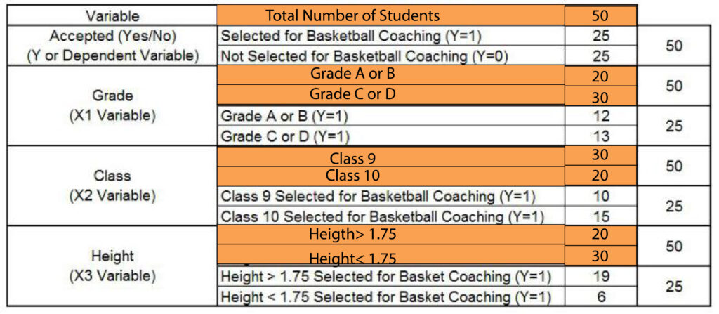
We have found that of the total, fifty students were chosen for coaching.
To Calculate Gini Index, we need to determine the ratios of these numbers.
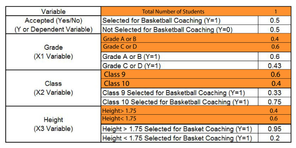
Then we can calculate how much Gini weighted Gini of SplitX1 (Grade) by formulating Gini for sub-nodes ‘A or B as well as ‘C or D.’ The calculations are as follows:
It is possible to use the same method for the X2 here, which is ‘Class”, and then find the Gini for splitting the ‘Class.’
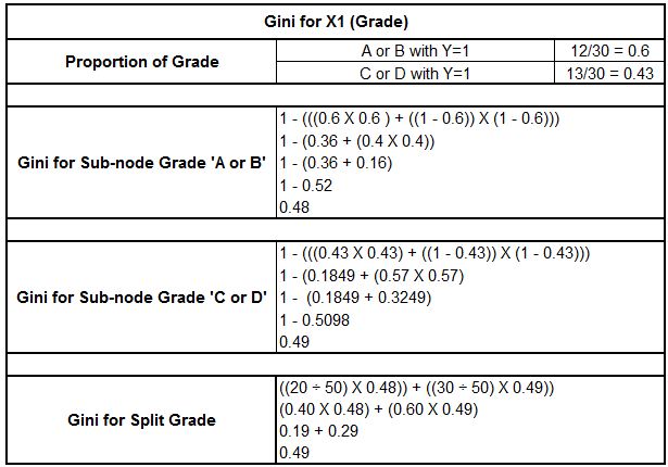
For X3 Height, which is a constant variable, The statistical software on the backend divides the variable into height > x and height < x. Then, it calculates the Gini value. Then, whichever value of x is able to provide the lowest Gini value is used to determine the Gini to split the constant variable.
In our instance, we can see an x value equal to 1.75, the minimum value compared to other height values, like 1.80 and 1.60. We discover this to be the Gini of split height turns at 0.23

Then we can look at the values of Gini and see that the minimum value of Gini is determined through height (0.23). Therefore, this variable is the root node and divides this data into two identical “purer” sets. The second value for the minimum Gini is determined for “Grade,” a variable. Lastly, the most significant number for Gini is found in “Class.” Therefore, the data is first divided by Height since it is an important factor in deciding if a child is selected for the basketball team or not.
Entropy
Entropy is a method used by ID3 which determines the amount of uncertainty within the data in order to determine the variable to divide. This is the one that requires less information to define itself. This is measured using the value of entropy. If the variable is homogeneous, then the value of entropy would be 0. If the variable is chaotic and has a symmetrical division, then the entropy value will be 1.
The Entropy formula is
H = -p log2p – q log2q
With P and Q being the probability of Y=1 or the probability of Y=0 for every variable.
(Below are the data we are using the basketball coaching data)
If we determine the entropy of the parent Node (Parent node refers to the part that is subdivided. The dependent variable here refers to the Parent Node), the result will turn out as 1. in our case, it is impure, with evenly divided groups (25 students chosen and 25 students not chosen)
The computations for this are shown below.
= -(25/50) X log2 (25/50) – (25/50) X log2(25/50)
= – (0.5 X -1) – (0.5 X -1)
= – (-0.5) – (-0.5)
= 1
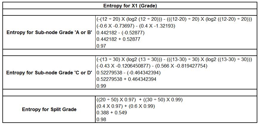
This is an impure node. Now we look for that root point. We calculate the entropy of different independent variables and determine the entropy for every independent variable included in the process. The first step is to determine the entropy of the variable x1, that is, grade.

We could similarly apply the same method to X2 and X3, which is height and class. Discover the entropy of Split the class as well as height.
Note: Since it is a constant quantity, statistical software uses entropy for each value and then splits according to the one with the lowest amount of entropy. Equal Size bins may also be utilized to reduce the time required to complete.
In comparing the entropy results, it appears that the split on height time should be the first step because its entropy value is the most minimal meaning that it offers the purest node.
Chi-Square
As stated above, Chi-Square is utilized in CHAID. In this case, the decision tree algorithm conducts a chi-square test and determines the chi-square values. The greater the value of chi-square, the more important the variable is when setting the split value. The exact calculation of chi-square is not the subject of this blog since it is already covered in the blog Chi-Square. Reading the blog to know the calculation process to determine the chi-square is recommended.
Metrics for Regression Trees
Reduction in Variance
If the dependent variable is continuous, we apply Reduction in Variance, which means that the variable is chosen for the split that provides the least variance. (refer to Measures of Variability for more information on the details of how Variance operates).
Formula for variation is
(x – x )2 / n
However, if you are dealing with categorical variables, it may become complex.
Below are the equations to determine the variance of the categorical variables that comprise our example: the X1 variable and then its X2 (Grade as well as Class). The variable x represents the value, and x represents the average of the variable, while the number n represents the total amount of records. The students have been assigned 1 for those chosen (Y=1) and zero for those not selected (Y=0). We won’t use the 1s and 0s in order to calculate the mean and deviation.
For example, let’s calculate the mean and variance for this root node. In this case, we will have fifteen 1s (y=1) and 15 zeros (y=0 ).
We calculate the mean by ((25 1) + (25 x (0)) 50, which equals 0.5
It is now possible to use this formula to calculate variance. In this case, x is 0.5. Then x will be 1 and 0.
There are 50 entries. The equation will read (x-x)2x 50/n
To be more precise, the formula could look like this:
(1-0.5)2 + (1-0.5)2 + (1-0.5)2 + (1-0.5)2 + (1-0.5)2 + (1-0.5)2 + (1-0.5)2 + (1-0.5)2 + (1-0.5)2 + (1-0.5)2 + (1-0.5)2 + (1-0.5)2 + (1-0.5)2 + (1-0.5)2 + (1-0.5)2 + (1-0.5)2 + (1-0.5)2 + (1-0.5)2 + (1-0.5)2 + (1-0.5)2 + (1-0.5)2 + (1-0.5)2 + (1-0.5)2 + (1-0.5)2 + (1-0.5)2 + (0-0.5)2 + (0-0.5)2 + (0-0.5)2 + (0-0.5)2 + (0-0.5)2 + (0-0.5)2 + (0-0.5)2 + (0-0.5)2 + (0-0.5)2 + (0-0.5)2 + (0-0.5)2 + (0-0.5)2 + (0-0.5)2 + (0-0.5)2 + (0-0.5)2 + (0-0.5)2 + (0-0.5)2 + (0-0.5)2 + (0-0.5)2 + (0-0.5)2 + (0-0.5)2 + (0-0.5)2 + (0-0.5)2 + (0-0.5)2 + (0-0.5)2 / 50
This could be written in (1-0.5)2 25 + (0-0.5)2 25 50
With this, we can eventually come up with an calculation (25 25 X (1-0.5)2)+(25 + (0-0.5)2) 50
The formula above can be used to calculate both the variance and mean of every variable. Look below for the calculation to calculate the variance of the X1 (Grade) variable.
It is possible to use similar formulas to determine the variance of the Split Class.

The results are comparable to those of the entropy, with the “Grade” being the most important variable since its variance is greater (0.24) than that of the categorical variables, which is ‘Class’with the same variance of 0.21. Its variance Numerical Variable follows the same pattern, and the variable that provides the least variance is considered the perfect split.
ANOVA
Analysis of Variance may also be used to split the sample, where we determine if the mean from two categories is comparable to one another or not. The split is performed for all variables. ANOVA is run for all subgroups of the variables. Then, the variable with the highest F value is used to divide the sample. To understand the intricacies of how ANOVA operates, refer to the section on F-Tests.
Parameters of Decision Trees
One of the main disadvantages of the decision tree is that it is highly susceptible to overfitting and could be complicated very quickly. For numerical dependent variables, they may be so complicated that it generates splits for each numerical independent variable, thereby creating one leaf for each data point within the information. To address this issue, the decision tree comes with a set of elements that may be tuned or tweaked to regulate the degree of complexity of the tree in order to prevent it from overfitting. (These hyper-parameters are available in programs such as GridSearchCV in Python and Caret or expand.grid using R).
Furthermore, a decision tree is a nonparametric approach that can work efficiently with less data compared to other modeling algorithms. However, there’s a significant issue when using decision trees: It exhibits an excessive bias and is underfit in certain areas of the data, while it exhibits large variance and becomes overfit in a few regions. This issue can be solved by employing methods like cross-validation of K-Folds, and group methods like Gradient, Bootstrap Boosted Trees, Random Forest, etc. This has all been studied within Model Validation and Ensemble Methods. In this case, we use different parts of the data to create multiple models so that the bias and high variance in some datasets are able to cancel one another out.
Because of the issue of the complexity (overfitting) and variations in bias-variance across various samples, we typically combine both for a cross-validated hyperparameter search to identify the most appropriate parameters to provide us with the highest complexity. We also make sure to use the correct number of subsets to deal with the fluctuations in bias-variance in various subsets of data (This is discussed within this Application part ).
In this blog post, we will learn about the different parameters available to manage the complexity of decision trees. They can be classified into two kinds – ones related to the dimensions of the trees to limit complexity and parameters related to pruning, where it employs a bottom-up strategy to create the decision tree.
Parameters Related to the Size of the Tree
Maximum Depth
The most simple parameter to comprehend is the maximum depth, which is essential in adjusting trees and models based on trees. It’s the longest distance from the root node until the leaf node or the depth of the layers that comprise the leaves. We typically assign a maximum number or depth limit for the model of decision trees to limit further splitting of the nodes in order that when the desired depth is attained, the tree ceases breaking up.
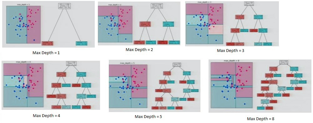
The partitioning of information at various levels of depth
In the example above, we have two components, one on the x and the other along the y-axis. This shows that the most efficient split can be achieved using the one-axis, x, i.e., divide the variable along the x-axis. Then, identify the value that will give the most effective result (the one with the lowest entropy or Gini dependent on the algorithm decision tree that it uses). If max depth is set to 1, it breaks the data and states that the data points on the left side will be identified as zero (blue or background color), but the actual 0 is blue dots. This makes the model too general and may not be a good fit for the model. But, if it keeps going and partitions all the information, it comes up with a different way to divide the data, and it creates branches and continues to divide the space. It is evident that at the point it reaches its maximum depth, it has all of the leaves, which are pure, however. This can lead to overfitting because it is extremely complicated and could produce unsatisfactory results when tested or when applied to new data. This is why we set the maximum depth to 5 for a moderately complex but accurate decision tree.
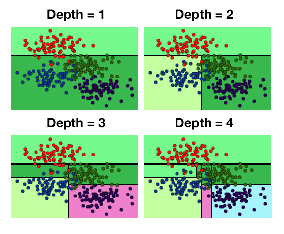
Division of data at various levels of depth
The increased depth of the model increases the difficulty of the model for decision trees.
Minimum Split Size
Another parameter by which we determine an acceptable number of observations required for the node to divide further. This is a way to control the overfitting and underfitting. A low number of the Minimum Split Size can cause overfitting, with only a few observations taken into consideration for further splitting; however, an extreme value could result in underfitting because a significant amount of observations that, if divided, can offer valuable insights will not be divided.
Minimum Leaf Size
In this case, we could provide an amount that determines the minimum number of observers that a terminal node should be able to. It can be used to determine the imbalance of classes. For instance, when we set the minimum split size as 99 and have a node that has 100 observers, the node is able to be split, but after splitting, we discover it is the case that child nodes contain 99 observations in one while one observer in the other. In ANOVA, we have explained and in other Basic Statistical concepts that each category of a variable needs to contain a minimum amount of observations that must be considered for any test in statistical research. In this case, we also determine an appropriate size for the leaf, which generally corresponds to 10 percent or less of the split minimum size.
The maximum amount of variables
The maximum number of variables a decision tree model could employ is a small number of features that can cause underfitting and a large number of features that can cause overfitting. Furthermore, they are chosen randomly, so if you have certain variables you consider to be important and would like to include in the decision trees, this parameter should not be suggested. In general, about 50% of features need to be considered; therefore, if there are 100 different features, the minimum number of variables could vary from 40-60, based on the information available.
Maximum Impurity
In the Maximum Depth, we saw how a very small number of depths caused areas with red spots to be regarded as blue. It is possible to restrict the number of false points that must be present in the same area before splitting stops.
Parameters Related to Pruning
Pruning is a bit specific to software as R allows it and incorporates it in group methods like XGBoost (package named the rpart), although Python’s sklearn package does not support pruning. However, a python user might argue that, as regards predictions, it is possible to use techniques like random forests, where it is not necessary to cut the decision tree in order to limit overfitting. If we are looking for an extremely simple and easy-to-understand model, then pruning a decision tree is a great option. In the past, the pruning process was the bottom-up method of creating decision trees, so if we’re using the top-down method, any split that produces negative results isn’t thought of, but, on the other hand, splitting it would provide us with a boost in precision that would have meant the initial loss could have been able to bear. (Similar to what was observed with Backward Elimination: Feature Selection). Pruning, however, results in general gains and losses when determining the nodes to be divided. Therefore, pruning is useful to increase the efficiency of the models.
Ensemble Methods of Decision Trees
Ensemble methods are discussed in their own sections. Still, to provide an idea of the possibilities, Decision Trees can be utilized in conjunction with Ensemble Methods which solve the issue of Bias-Variance. When it comes to a decision, the most frequently used Ensemble techniques are increasing (particularly Extra Gradient, Standard Gradient Boosting also known as”XGBoost”) along with Bootstrap Aggregating or Bagging (particularly a variant of Bagging that is known as Random Forests ). For more information about them, look through the ensemble techniques.
Decision Trees are one of the most effective tools that can be utilized to solve Regression as well as Classification Problems. It is simple to build and comprehend. Contrary to other available algorithms for learning, this one gives the user more control over the entire process. This is accomplished by allowing users to choose from several algorithms, hyper-parameters, etc. It is able to visualize the entire process and, in turn, assists in giving the user an understanding of the way the algorithm operates. Learning to master Decision Trees can provide insight into the data that other model-based algorithms cannot. We have many ways to create Decision Trees, and in this article, we only looked at the most popular.
