Regression is terminology in statistics that is used to determine the relationship between two variables or to quantify the relationship between independent variables to their dependent counterparts. This blog article will explore Linear Regression, where the relationship between the independent and dependent variables is linear. When the connection between two variables isn’t linear, other kinds of regression can be utilized; however, to use linear regression, it is necessary to take into consideration a very solid assumption that all independent variables are dependent in a linear manner on that dependent variable. In addition, to allow Linear Regression to function, all variables must be continuous (interval/ratio adjusted).
Use of Linear Regression
What is the reason why Linear Regression is used in other statistical techniques? The reason is that constructing an equation for linear regression can aid with more complicated questions. Linear Regression helps in two ways. To clarify this, two scenarios are possible to consider.
Scenario 1 A car company intends to expand into the country you reside in and is looking for a city in which it will establish the first of its dealerships. The company has information where their sales are available for various variables (independent variables). This is where Linear Regression could be helpful, as it can clarify which factor plays the largest part in deciding on the place for the store.
2. The company of a car plans to introduce a new version of an in-use vehicle. They’d like to know the extent to which a decrease in cost and an increase in mileage will cause the sales to increase by a factor of two. In this case, Linear Regression can provide precise figures upon which the business can decide the price and begin an engine improvement process to improve the vehicle’s mileage.
Therefore, Linear Regression provides us with the variables that are crucial and provide us with the values that could be utilized to predict the dependent variable.
Types of Linear Regression
There are two kinds of Linear Regression: Single Linear Regression as well as Multivariate Linear Regression. The first step is to discuss the mathematical concepts using Single Linear Regression as 2-Dimensional Scatterplots are a great way to explain the calculations that the statistical software performs at the backend when developing the Regression Model.
Single Linear Regression
Simple Linear Regression is done when we have two variables: one dependent variable and one independent variable. For example, let’s look at an information set where the earnings of different dealerships are listed and the number of vehicles sold in their showroom. The dependent variable here is called ‘Income,’ and the independent variable is ‘Sales.’ When we look at these two variables, it becomes apparent that the two factors are negatively connected, and the amount of income is determined by sales.
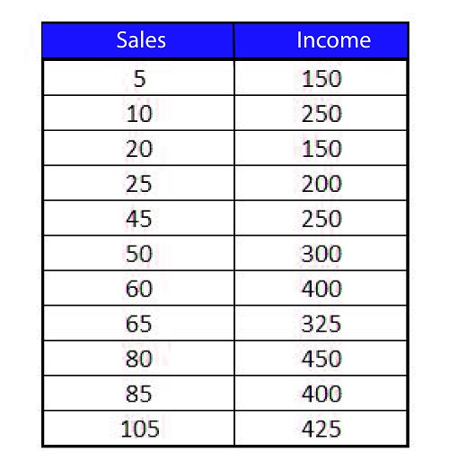
In the event that we graph it on a scatterplot, we will get an image like this:
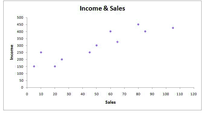
In the process of Simple Linear Regression, we are unable to make use of Linear Regression to find the dependent variables that are crucial because the only independent variable is but the other issue – the predictive one is solved when we can determine that the X value of sale and how much income could be anticipated. To determine the predicted value, a regression line is constructed that allows us to estimate how much Y will cost for the value of X.
This regression line follows an equation that follows:
Y = a + bx + e
where,
A is the y-intercept
B refers to the beta amount, or the standard regression coefficient or gradient of the line
x is the value for the independent variable
“e” is an error word.
Before going into details, Let us first understand the mechanism behind regression.
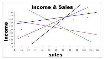
There is a dataset and the need for a regression line to determine the value of Y for X given. Let’s draw a line on the scatterplot in order to comprehend why we need to identify the correct lines of regression (good fitting).
We can see that a variety of regression lines could be made, but there will be only one line that will provide the most accurate prediction. Better prediction is a better predictor of error, and that’s what the Linear Regression Model does when it utilizes its Ordinary Least Square Regression to generate this regression line. The regression line represents the expected value, and the distance between lines and data point is the error. If we take the square of the distance and add all the squared distances, what we get is called”the sum of the squares.” It is also called”the total of squared deviations. The regression line in OLS regression will be drawn when the line yields the lowest amount of squares.
Calculating the Regression Equation / Best Fit Line
We can comprehend how this line is determined in three ways.
Intuitive Way
First, there is the intuitive way. In this case, we utilize a statistical program, and in the backend, the program begins to calculate the slope of this regression line. It also explores various combinations and permutations with different types of lines, such as negative slope, low slope, and so on. It then ends with a line that the sum of square errors is the smallest. This is because the different lines have a distinct distance to that data source. Lastly, the “Best Fit Line” is chosen where it is the case that squared variances are minimal. Using this method, the program can provide us with the intercept and the beta value.
Mathematical Way
Second, there is the Mathematical method. It is possible to use specific statistics to calculate beta coefficients, including mean, standard deviation, correlation, and mean coefficients.
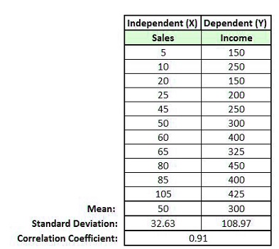
Then we can apply an equation to calculate how much beta (regression coefficient)

where,
The beta value is b,
The correlation between the variables X and Y,
Sy standard deviation of the Y variable,
Sx standard deviation of the X variable.
By using the formula above, we can determine the beta value.
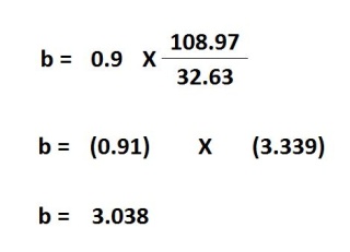
This is referred to as a standardized regression coefficient since, for example, the two variables we have are on different scales and have different standard deviations. In order to easily compare variables with each other, it is possible to create regression coefficients in which correlation coefficients are multiplied by the standard deviation, thereby converting the correlation coefficients into scales of measurement. (How the correlation coefficient differs from simple linear regression will be explained in the final section of this article). A standardized coefficient for regression could also be referred to as Regression Coefficient. It is also known as Standardised Coefficients, Beta Coefficients, Beta Value, the B0 value, and Weights.
After we know an estimate of beta, we can determine the alpha value, also known as the y-intercept. This can be calculated with the mentioned formula.
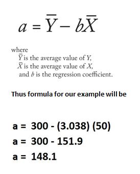
The value of the intercept of 148.1 is that, once the value of the x is predicted to be zero, The value of y will be predicted to be 148.1
y = A + BX
The y value is 148.1 + 3.038 x 0.
y = 148.1
But, this isn’t accurate and may be too optimistic. This is why an additional error component is included in the formula. The simple formula for the Y formula is Y = A + BX (same as the formula y = a + Bx and that y = mx + c). The formula that incorporates the error component could be expressed using two different ways one way
e = y – y
or
e = y – a+ bx
(here, the bx + A =y indicates the predicted value of y)
Thus, we use two regression formulas, one for the predicted value of the y variable and another that is based on the actual value of y. The error can be identified and can be incorporated into the estimation.

So, we can estimate the Y value based on the value X. For instance, if the person’s sales are 55, then we can predict the earnings. The answer is
y = A + BX
The y value is 148.1 + (3.038) (55)
y = 315
So the earnings for sales of 55 is 315 minus/minus the error term.
Another way to understand the regression coefficient of 3.038 could be to say that, for growth in sales, keeping all other variables equal (for more than one regression), the profit will increase by 3.038.
Finding Best Fit Line in Graph
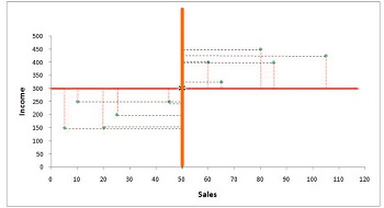
To determine the most suitable regression line, we first create an x-axis graph with the independent variable and the y-axis containing an independent variable. Then, we find the average of these two variable in the graph.
As you can see below in the figure, the mean of these two variables crosses at a certain point (where the average of both the independent and dependent variables intersect). This is the place through which all regression lines need to go.
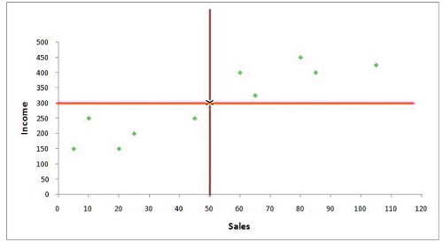
The next task is to determine the intercept value, i.e., the y-axis point where the regression line passes, giving the minimum sum of residual/square error/sum in squares/summation of deviations squared.
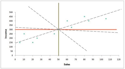
There are a number of possible lines that could pass through the intersection. Therefore, we must find the location where the line crosses the y-axis.
The distance from the x to the mean value for all observations is calculated to calculate the intercept value. The same process can be done with y. In this case, the distance of every observation from the mean of y is determined.
So we get the difference in both variables’ values from each of their mean values. (x+ x and y-y) Then we square the difference in the independent variable’s value from their mean and then sum the results ((x* x)2). Then, we multiply the difference in the x values from their mean and add the difference in the y values from their mean, and then sum them ( (x+ (x)( the y and)).
For this part, the words that will be utilized are b0, where the word b0 (pronounced as beta and not) is an abbreviation for intercept, and b1 is the beta number. Thus, the equation to calculate the regression line is y = b0 x b1x.
To determine how much beta is (i.e., that is, the slope of the regression line), we can divide (x+ on)( the y and) by (x* x)2, and then we have the beta1.
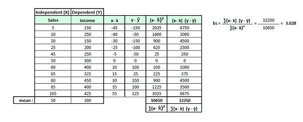
We can now determine the B0 (intercept value) using the existing values of the equation.
The equation for the regression line can be described as y = b0 +.
The y here will be equal to the average of the y variable, and the x is the average of the x variable.
We employ these numbers since a regression line needs to travel over these coordinates (300,50). Therefore, your equation is
300 = b0 + 3.028(50)
It is possible to shuffle the equation to get the b0.
300 = b0 + 9.084
300 – 151.4 = b0
148.6 = b0
It is now possible to sketch what we call the Best Fit Line using both points. (The intersect of the median of the x and y variable, and the intersection).
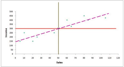
There are various methods to identify the most efficient regression line. The points that are on this line are the expected values for a certain value of the variable x.
Simple Linear Regression v/s Correlation
Correlation is the term of relationship, how two variables are related to one another but do not differentiate between dependent and independent variables; however, when using Linear Regression, there is always an independent and dependent variable in which the value predicts the values of the dependent variables for the variable in the independent. The linear regression output in most statistical programs provides us with details of which variables are connected to one another. This means that it is evident that the Correlation coefficient (r) is identical to the Linear Regression Coefficient (b), with the only difference being in the fact that the Regression Coefficient is now standardized. But, running a Linear regression can be more beneficial in certain ways since it is able to determine the worth of the variable in question. There isn’t much difference between simple Linear Regression or Correlation. The true benefit of regression can be derived by employing multi-linear regression.
Multiple Linear Regression
Multiple Linear Regression works the same as Simple Linear Regression; however, it contains multiple independent variables. For instance, if you add another variable, “experience” in the case above, then we’ll have two independent variables:’sales as well as experience’. Both variables will each have their own coefficient of regression, which can be used to determine the significance of the dependent variable.
In this case, however, the regression line isn’t constructed; rather, an appropriate hyperplane is constructed.
A Line of Best Fit is created in Simple Linear Regression, while in Multiple Linear Regression, a Plane or Hyperplane of Best Fit is constructed.
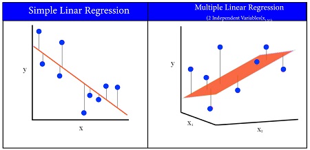
The formula for the regression plane (having two independently variables) will be
Y = a + b1x1 + b2x2 + e
where,
A is the y-intercept
Beta is the value of b1 or the standardized regression coefficient for the variable “x1”
The value of x1 is the independent variable “x1”.
Similar to b2 to b2, it is the beta value or the standardized regression coefficient for the variable “x2”
The value of the independent variable “x2” is the value of the independent variable.
E is an error word or random error/noise
Y is the dependent Y_Variable/response variable that will have a value that can be predicted.
For Simple Linear Regression, we discovered an error that meant we could not explain variance in our dependent variable using only one independent variable. This means that other variables, such as the predictor variable called ‘Experience,’ can help explain an individual’s earnings. When we mix the car sales of a dealer with the knowledge he has in the business world and business, we might be able to decrease the error rate by explaining more variance in income. In order to decrease the unexplained variation, i.e., error, we include variables that enhance our predictions.
This is why Multiple Linear Regression provides us with beta values for multiple independent variables as well as, like ANOVA, it tests the degree to which an independent variable can be linked with the dependent variable after taking into account the other variables that are independent and describes how much each independent variable is connected with the dependent variables.
Regression Modeling
Linear Regression and, in particular, Multilinear Regression is used in Regression Modeling when we have information and must predict the values of the dependent variable. In this case, for example, We have 10 variables independent of each other. We incorporate the 10 independent variables within a static application to build the regression model, obtain the beta coefficients, the intercept and error term, and then use this equation of linear regression in order to determine the values of dependent variables.
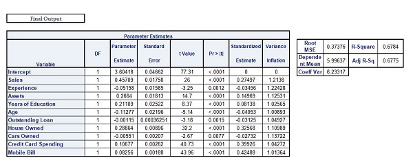
Therefore, a regression model aids in making predictions about the dependent variable’s value for a given value from the dependent variables. But it’s important to recognize that the process doesn’t end simply by constructing an equation. There are many variables to be considered, including multicollinearity as a problem and related concepts like overfitting and underfitting the model. To fully comprehend this, concepts in statistics like R square and Adjusted R square and Adjusted R were studied. Also, we must look into issues like Heteroscedasticity as well as Auto Correlation and other issues that are that are encountered in Linear Regression models. This is why we have to assess our model. These are discussed within the post Model Evaluation of Regression models. The ultimate goal of developing models is to test them against unobserved data. For this, we need validation of our model to make sure that the variables in our model that are important and their associated coefficients are the ones that can give us the best results in predicting the values of data that is not known (i.e., that data with which the model hasn’t been constructed). For this, various approaches have been studied under the heading model validation.
