Outlier treatment is an additional procedure in the pre-processing of data. It can be done prior to missing value Imputation (one might choose to perform missing value treatment before outliers have been treated, particularly if you are using mean imputation since outliers could affect the data). Outliers are an observation at an unnatural location from others or any observation that is not in the bulk of data or from the overall pattern. Outliers may be mild and extreme, with the extreme far from the source by a significant amount. Additionally, an outlier could be found in each of the variables (Univariate Outlier) or can be viewed with the other parameters (Bivariate Outlier ).
As explained in The Measures of Central Tendency and Measures of Variability, an outlier may adversely impact various statistical models, with specific machines and statistical models being extremely susceptible to outliers. Outliers can arise by a variety of reasons, like inefficient or incorrect data collection or data entry errors such as human errors that occur when entering data into a spreadsheet, industrial machine malfunctions in which the machine malfunctions and eventually reflect inaccurate values in results, measurements errors in which the data is supposed to be in specific measurement unit (e.g., Kg) is displayed in another measure (e.g., grams) or sampling errors when sampled from the group that isn’t in question (such when analyzing the salaries of teachers in schools and industrialists’ income is included) and also intentional Outliers such as fraudulent retail transactions, or even with false information about themselves or their customers. Natural Outliers where a fault or bias does not cause the outlier; however, it is a natural phenomenon (for instance, when taking an income sample from several teachers, certain teachers from private schools have a higher income than others, and the earnings of these teachers could be described as a natural outlier. ).
Method for dealing with outliers
Deleting observations
This is the most straightforward method to treat outliers. The rows that contain an outlier can be deleted, but the main disadvantage of this method is that there could be a significant loss of data if there are many outliers. Outliers could be located within a specific variable in an entire dataset. When we delete the entire row, we will lose information for additional variables (features); consequently, outliers are restricted by using various techniques.
Relating observations
There are many ways by which outliers can be detected and capped by adding observations. Capping outliers can be accomplished by using boxplots, quantiles, standard deviation, quartiles, and so on.
Boxplot
Understanding Boxplot
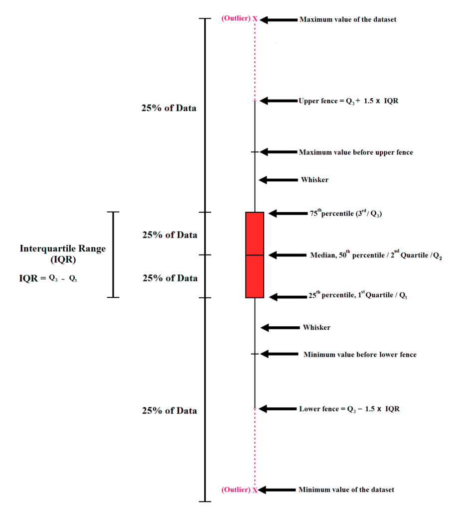
We can visualize the data points and see the outliers further away. But, they aren’t often used since they take a long time to limit outliers with boxplots when there are many aspects in a data set. Other methods, like standard deviation and percentiles (discussed below), are reliable. In general, when creating boxplots, lots of data is needed. If there is an error in capping outliers, we must go back to the boxplot repeatedly. This is why boxplots are utilized in situations where precision is required, like the risk model, chemical trials, or risk modeling. It takes weeks to complete the data. However, in other fields like Marketing Analysis, etc., other methods can be equally reliable.
Quartile Ranges
In a data set, the most extreme points in a data set are thought to be three times interquartile variance, which lies below the first, or higher than the 3rd quartile. Mild outliers are in the range of 1.5 times interquartile interval, below the first quartile, or above 3 quartiles.
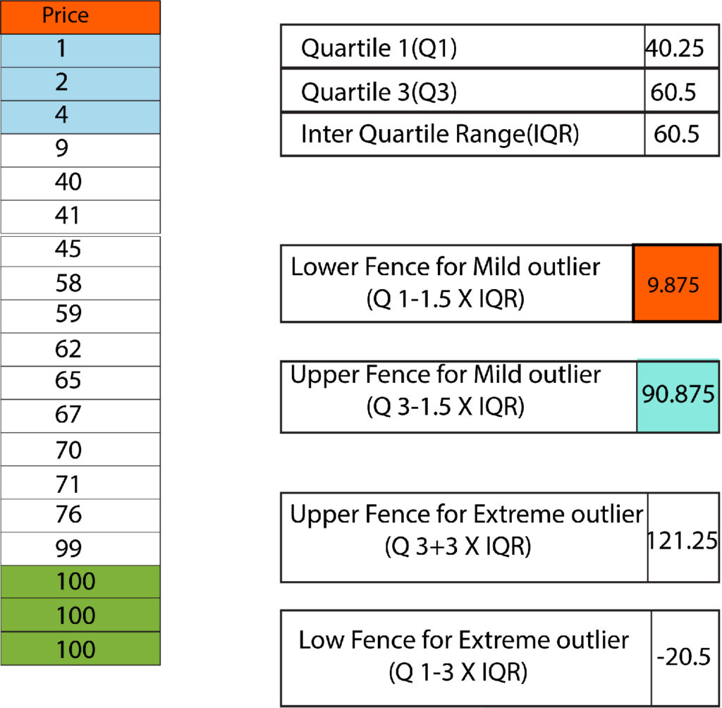
In this data, we see several minor outliers. In this dataset, any value that exceeds 90.875 is capped at 90.875, and any value less than 9.875 will be limited to 9.875. In this dataset, we did not detect many extreme extremes.
Quantiles / Percentile
There are a variety of percentiles to choose from that range from P1 to P99. An unspecified value may be chosen for each variable based on when the percentile drops or increases dramatically. Before diving into this, you must understand the distinctions between quantiles, quartiles, and percentiles.

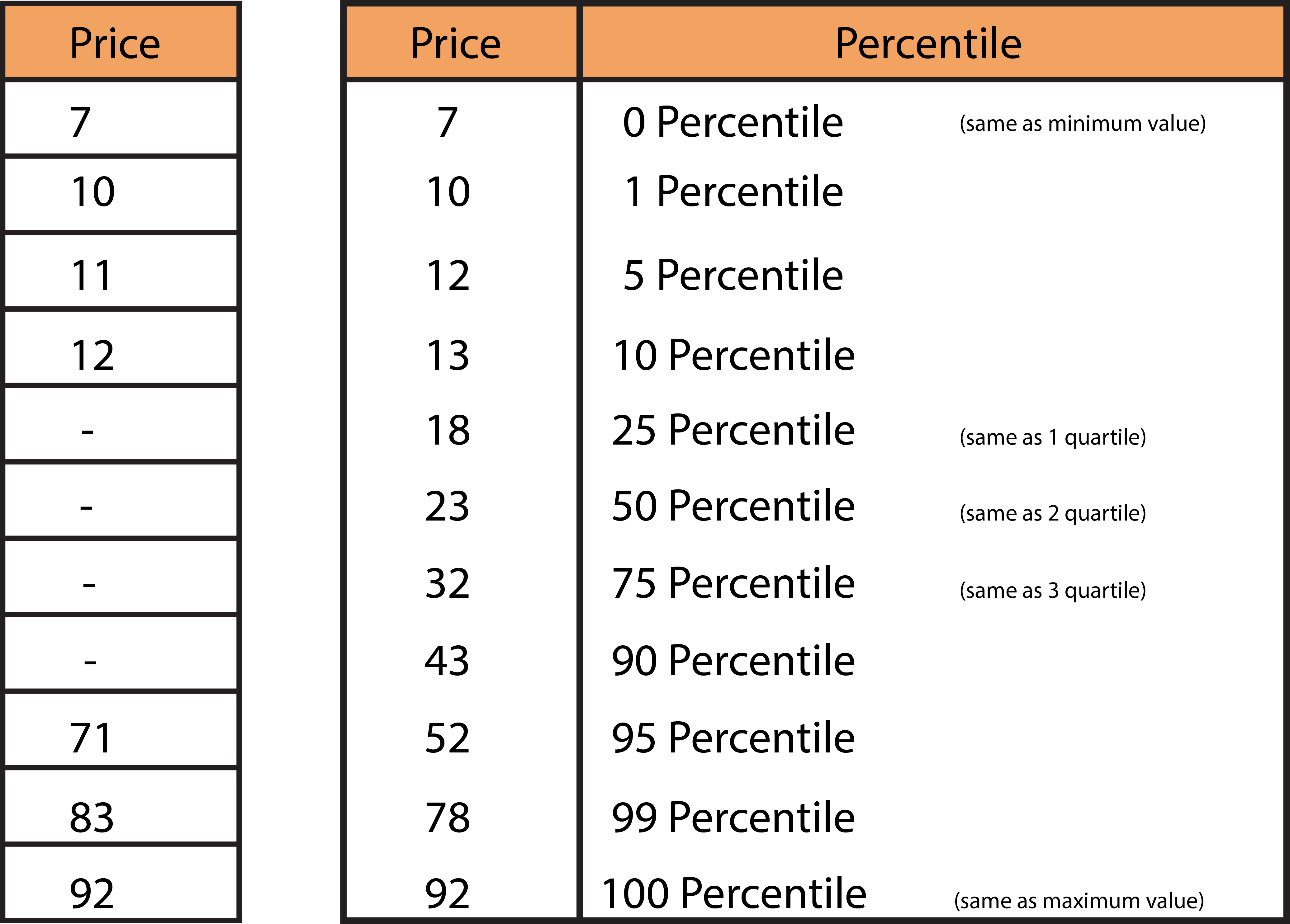
0 quartile = 0 quantile = 0 percentile
1 quartile = 0.25 quantile = 25 percentile
2 quartile = 0.5 quantile = 50 percentile (median)
3 quartile = 0.75 quantile = 75 percentile
4 quartile = 1 quantile = 100 percentile
We can see that there is an increase of sudden magnitude in the value of 95 and 99 percentiles; therefore, we can use the 95 percentile value, which is 52, to define the extreme values at the top. However, there isn’t a significant drop in the low values, indicating no excessive values (outliers) at the lower tier.
Standard Deviation
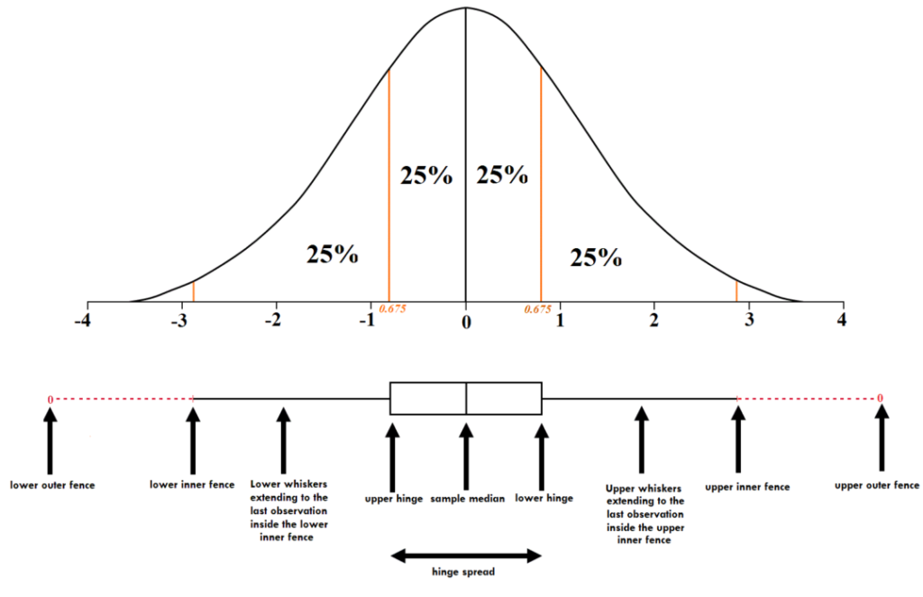
Another method for limiting outliers is to use standard deviation. In general, data is limited to two or three standard deviations higher than that of the average. For instance, if there is a variable, we can determine the standard deviation, multiply it by two, and subtract it from the mean; we’ll get a value lower than the upper limit. Adding this number to the mean will give us higher limits. A similar process can be applied to 3 standard deviations. In this case, we divide the standard deviation by 3 instead of 2.
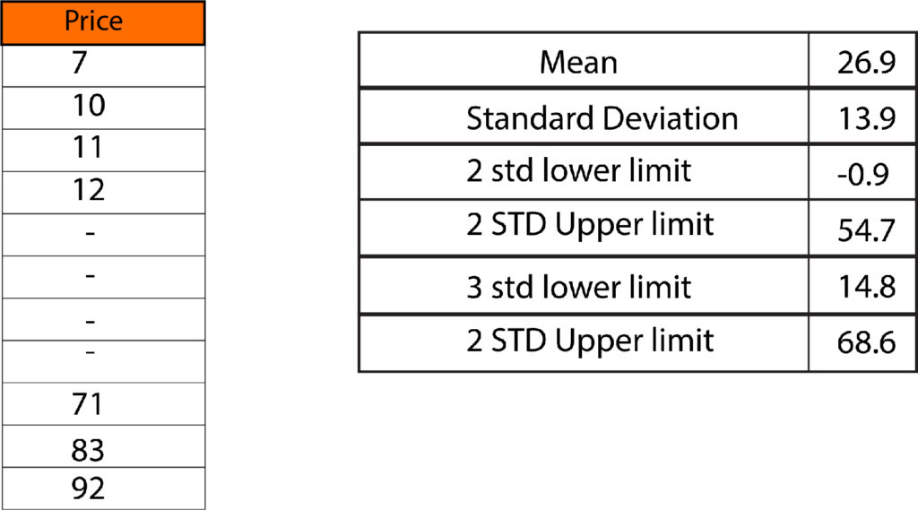
If you look at the same data set, the results appear to be like percentiles, in which we used 52 as the top value. We also didn’t see the lower extremities of any values. But, it is difficult to choose between the various STD levels; for this reason, frequency tables can be utilized when the amount of data is important. For instance, if we choose two std, we’ll have 5% of outliers, while using 3 std, we can discover 1% of outliers. In the case of outliers, discretion is essential. For this example, 5% outliers are an adequate number of outliers. However, there is a possibility that if we had discovered 10% outliers that had 2 std, this could have indicated that there are extreme values, like the price of a product, which could be costly. In this case, it is possible to choose another std number such as 2.5, and see what proportion of data is classified as an outlier. In real life, it is possible to limit outliers with 3 std; the use of 2 or 2.5 mean a significant number of records to be considered an outlier, which means it is not of good quality, which means that the data is not of high quality.
Methods like clustering can be utilized when the data is not in the clusters, could be considered, but it takes many hours and is employed to achieve high precision. Data transformation and Binning the data help in limiting the impact of outliers in data. But, the methods mentioned above are the most popular ways to control the negative impact of outliers.
