One of the initial steps in pre-processing is to combine the data sets so that modeling can be performed since the necessary data is scattered across different datasets and must be consolidated. Before any consolidation is possible, the variables must be identified. The method of identifying variables involves identifying the Predictor and the Target variable. The predictor x-variable is the input, and the target y-variable is the Output. For instance, there is a data set that includes variables such as the subject’s income, the amount of debt pending as well as whether they own a house or not, if they are married or not, and whether the subject was unable to pay loans or. The Target variables are whether the individual is incapable of repaying the loan or not. Other variables can also be used as input variables or predictive variables. The selection of the variable that is the target is essential to consolidate the data.
The data can be combined in various ways. Two methods will be covered:
- Appending
- Merging
Appending Datasets
Appending is a method for consolidating data sources so that information from multiple datasets can be merged vertically. Appending is typically required when the same information is scattered across multiple datasets. One typical situation is when information is kept in spreadsheets. Because they have a limited storage capacity, several spreadsheets could be there. Their data may be required to be added or ‘concatenated to ensure it is possible to analyze the data conducted.
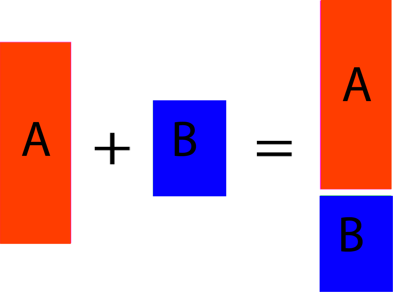
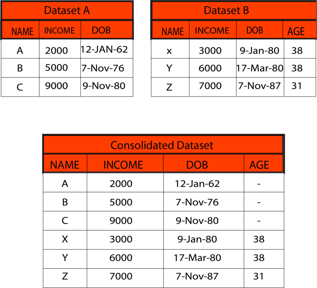
Appending heavily depends on the names of the variables. Each piece of information is “stacked” upon each to create an appended database. This is important to remember that in certain programs, the appending process can depend on the case. If you have two data sets wherein data set A contains three variables NAME, ‘INCOME’ as well, as ‘DOB.’ However, in dataset B, the three variables are named Name, Income, and DOB. In actuality, the name variable contains the same data. Still, because the process is case-sensitive and case-sensitive, the data in the variable named ‘Name’ in dataset B won’t be put in the same pile as the data from the variables ‘NAME’ in A.
Additionally, an appending process needs the columns to match. If there’s an additional variable in either the data that could affect the appending process, it may have to be forced.
Merging Datasets
Merging is a method of consolidating data wherein the data are merged horizontally. In this case, the variables are added to existing observations, i.e., moving the columns of one database to the next (unlike appending in which rows were transferred) in which the data sets are added to each other.
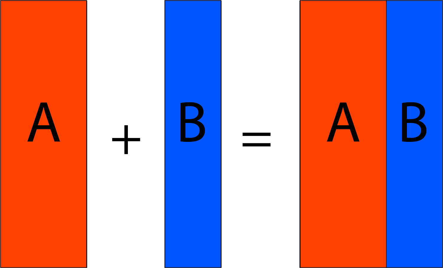
It is crucial to remember that at least one common variable must be present in both data sets and could be required to share the same name across both data sets (this requirement depends on the program you’re using). Multiple common variables may also be utilized during the merging process.
Common scenarios in which merging is needed when for instance, there are customers whose information about the demographics of the patients are accessible in one dataset, but the transaction details are accessible in a different. Customer name or the ‘Customer ID’ is the common variable, and the two datasets can be joined/combined/merged into one by using this common variable. This dataset can be used for further analysis and modeling.
To fully comprehend the process of merging and the results, It is important to comprehend the various types of relationships that the two datasets could have. There are generally three types of these relationships:
- One-to-One Relationship
- One to Many Relationship
- Many to Many Relationship
One-to-One Relationship
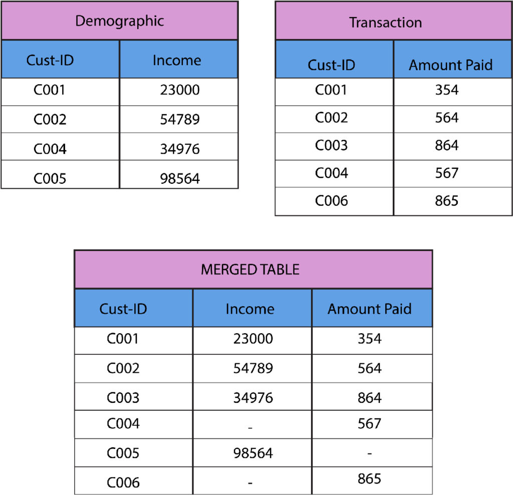
One-to-One, The relationship between two datasets, is created when for every one of the values of a shared variable from the first set of data, it is the only identical value for that same common variable in the second data set.
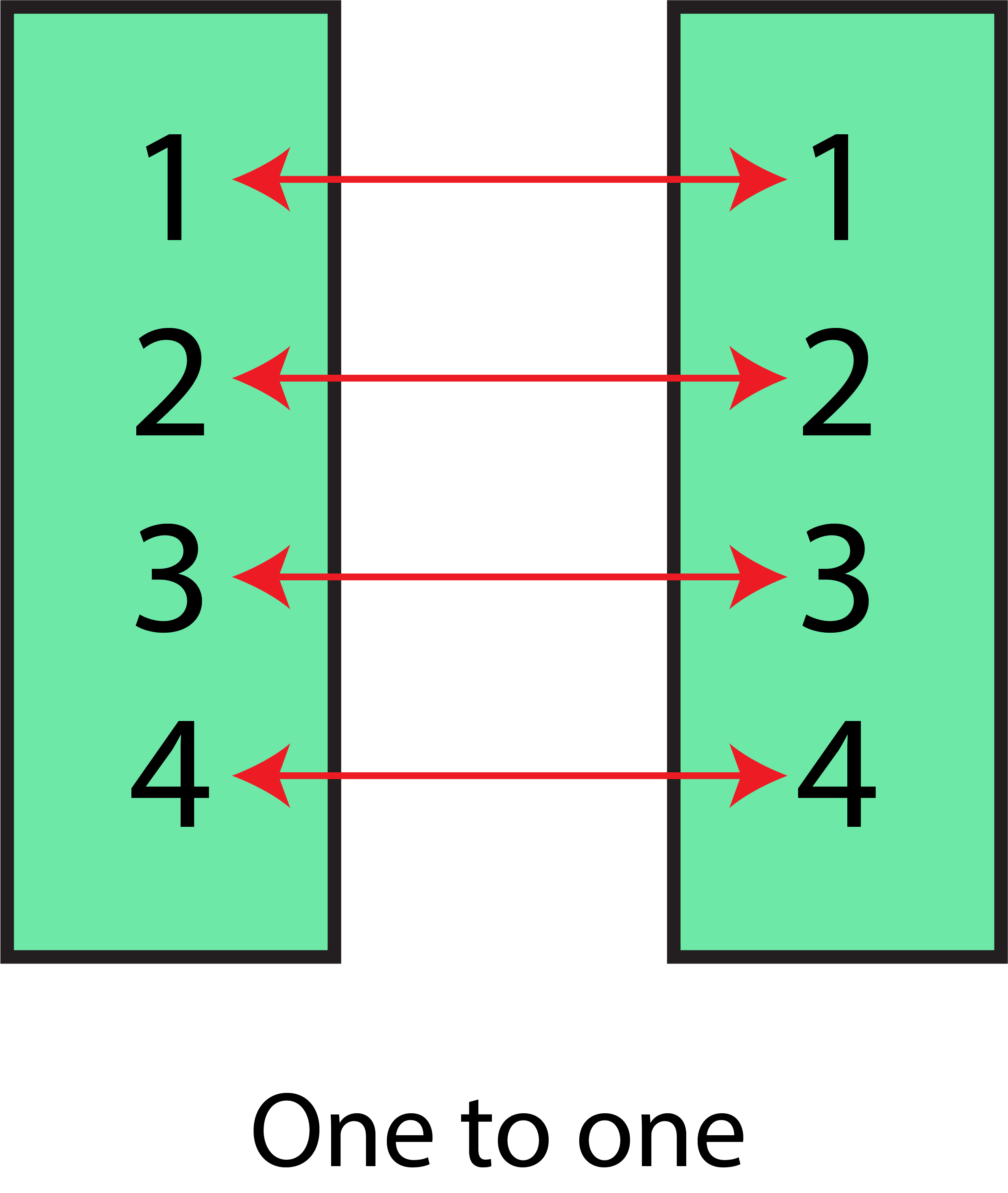
In this case, for instance, we have two databases wherein the demographics of customers in dataset A are given, and details are provided. In dataset B, we have transaction details for the customers. We need to combine the two datasets to create one complete database where the details of the demographics and transactions of every customer are provided. In this case, both datasets have a One-to-One relationship.
One to Many Relationship
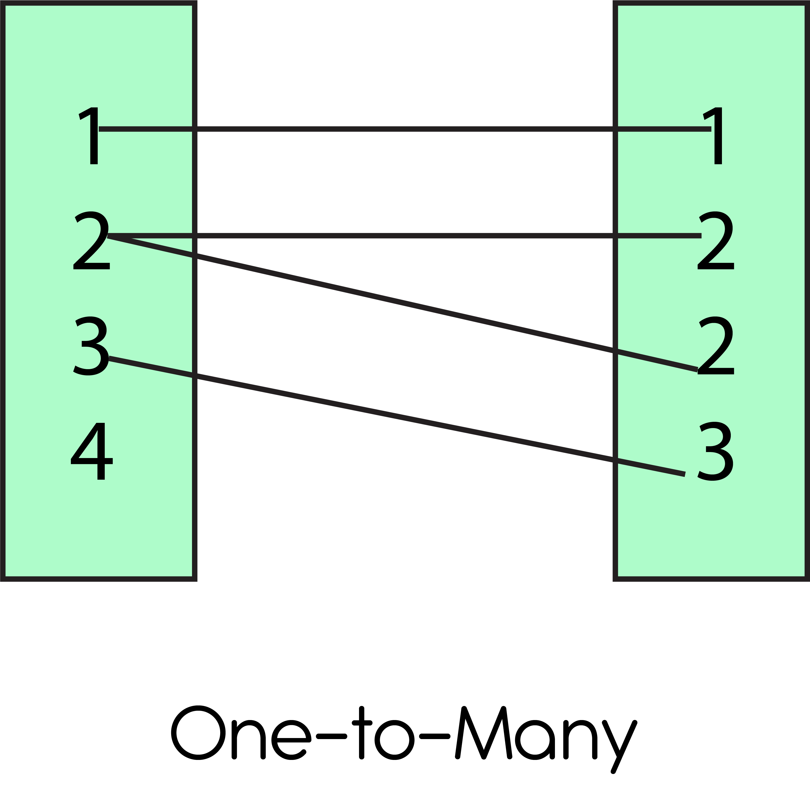
One-to-Many, The relationship between two datasets is created when for every number of common variables from the first set of data, there is more than one identical value for that same parameter in the secondary data set.
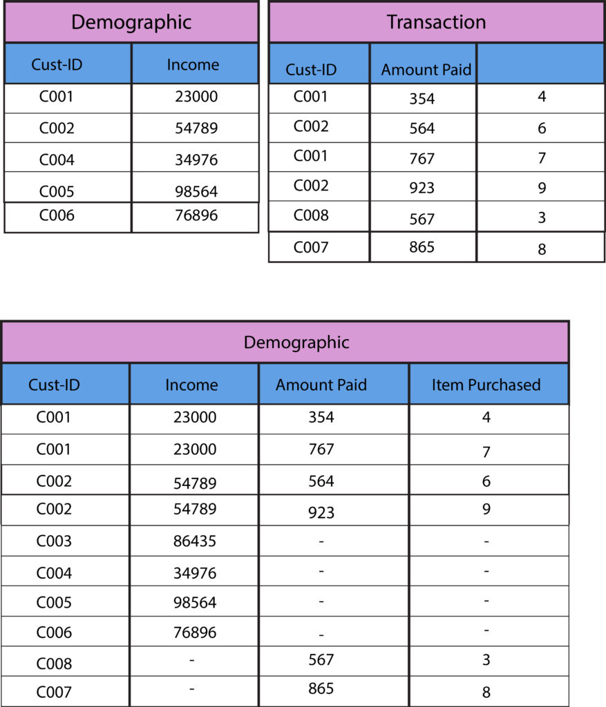
In this case, for example, there exist two datasets. In dataset A- information about their demographics is provided for each customer’s unique ID, and income details are provided; in the other dataset, transactions details are available that include considerable amounts of money paid and the number of goods bought for each customer ID. In this case, we need to join the two datasets to have a comprehensive dataset that includes each customer’s transaction and demographic details. In this instance, we can see both datasets have a one-to-many relationship.
Many to Many Relationship
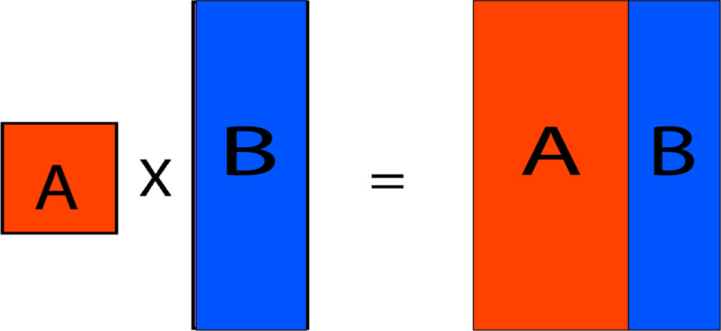
In a multiple-to-many relationship, the observations of every field (which can be used to establish an association between two data sets) are included several times in every dataset. Moreover, we need to join data horizontally so that the output includes all combinations of the observations, i.e., a cartesian result of rows. In this case, suppose if you have two tables that contain 2 and 3 records, respectively, in our Cartesian output, we get an array of 3 X two = six records.

In the following example, we will observe what happens when two data sets are combined to create a Cartesian item.
The problem with the many-to-many relationship is that we obtain the row-based product; therefore, we are able to count the same row multiple times, which results in duplicates in the output data, which can result in inaccurate results and can result in the loss of computing resources like processing speed and space.
Ways of Joining Tables
There are various ways to join tables, including Inside Join, Left Join, Full Join, Right Join, etc.
We can comprehend the different ways of using HTML0 by using an example that shows two sets of data: Dataset A and Dataset B.
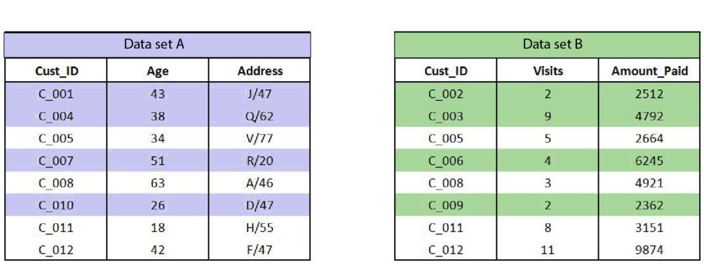
Highlighted observations include those that the Cust_ID only found in this particular table and is not associated with any other table.
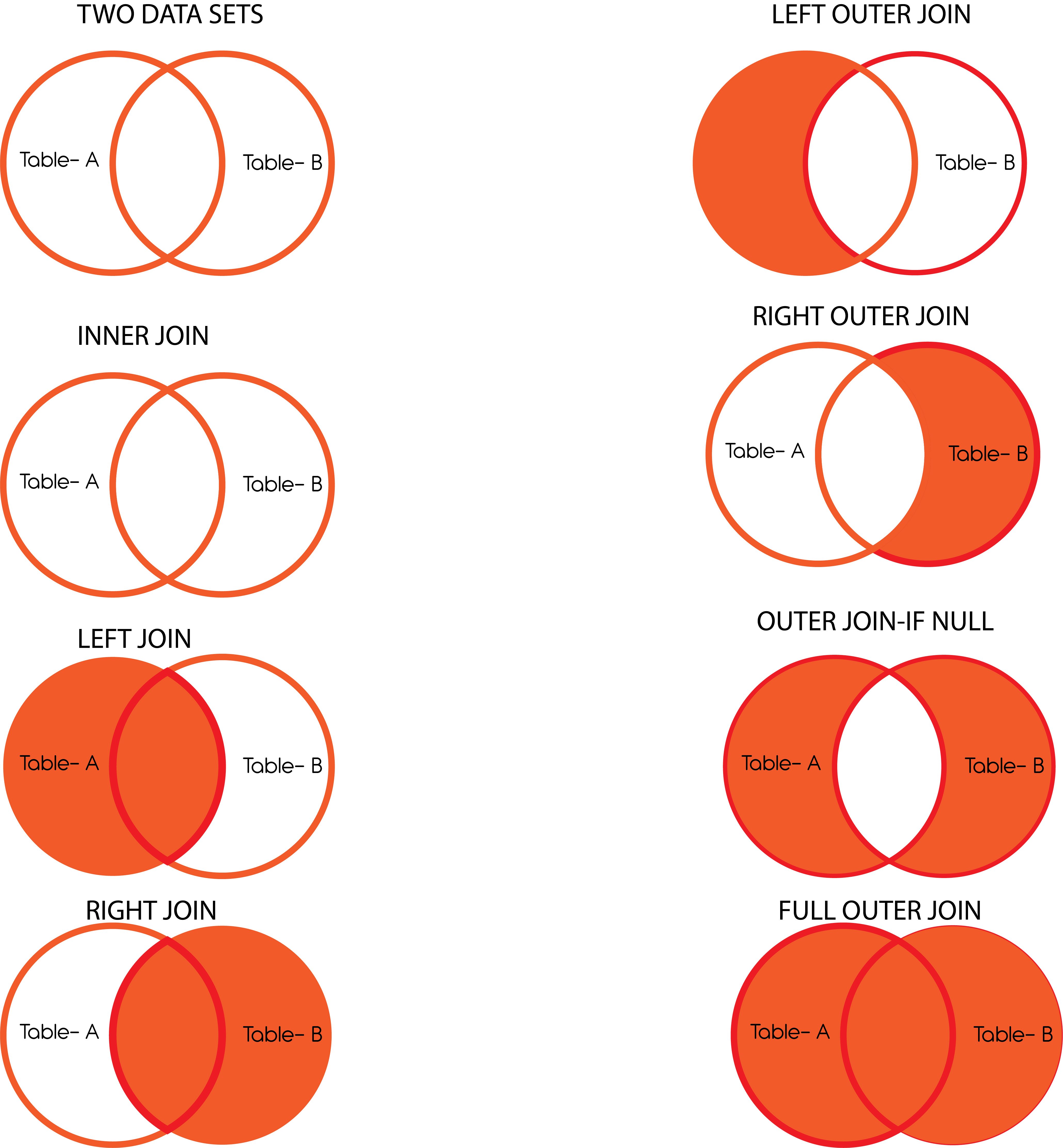
There are a variety of methods of combining the two sets of data.
Inner Join
Here, only the common records from both data sets are taken into consideration.

Left Join
Each observation included in Table-A, along with those observations shared in Table B, is considered. (A = 1 , B = 0)

Right Join
Every observation listed in Table B, together with those similar to Table-A, is considered. (A = 0 , B = 1)

Additionally, there are outer joins that can be utilized. Some terms like right Join or Right Outer Join can be used interchangeably. However, when we refer to Outer Join, we refer to (in SQL terms), in which we insert the clause “WHERE Left_Table.ID is NULL’, which means that only records specific to the right table will be included within the result. There are four kinds of outer joins: Right Outer Join (is null) and Right Outer Joint (is null) Outer Join (is null) and Full Outer Joint.
Left Outer Join (Is Null)
Only observations specific to Dataset-A are taken into consideration. (A = 1)

Right Outer Join (Is Null)
Only those observations which are specific to Dataset-B are taken into account. (B = 1 )

Outer Join (Is Null)
Sometimes, it is referred to as Outer Join; here, only the most unique observations are considered. (A = 0 , B = 0)

Full Outer Join
Here, all observations from the whole collection are taken into account. (A = 1 , B = 1)

In merging, using one variable, information is searched for in a different data set, and in the process, data is added. This is where the increase in variables is made.
It is crucial to remember that observations may be duplicated, for example, in a Left-Join. Observations are overwritten to table A when you have more than one shared variable within both datasets. So, no common variables must exist in both data sets unless the variable is by which data is combined.
Data sets are consolidated, a typical process that occurs in the process of preparation. In this article, we explored two methods to consolidate data sets: Appending, where data are added to an already existing database (or an entirely new one has been constructed), and merging, where new features have been added to the existing dataset. Both approaches are equally effective and utilized based on the particular situation. After the data sets have been consolidated, further pre-processing procedures such as Missing Value Treat and Outlier Treatment, as well as other Feature Engineering steps, can be applied to ensure that the data is clean and suitable for an algorithm for learning.
